R visualization: barplot with chisqure test by ggplot2
grouped barplot with chisqure test
Introduction
chi-square test is used to test whether there is a significant difference between categories. Here, we combined barplot and chi-square test to display these results.
Loading required packages
knitr::opts_chunk$set(message = FALSE, warning = FALSE)

library(tidyverse)
# install.packages("titanic")
library(titanic)

# rm(list = ls())
options(stringsAsFactors = F)
Data preparation
- Data object from titanic R package
dat <- as_tibble(titanic_train)

head(dat)
## # A tibble: 6 × 12
##   PassengerId Survived Pclass Name    Sex     Age SibSp Parch Ticket  Fare Cabin
##         <int>    <int>  <int> <chr>   <chr> <dbl> <int> <int> <chr>  <dbl> <chr>
## 1           1        0      3 Braund… male     22     1     0 A/5 2…  7.25 ""
## 2           2        1      1 Cuming… fema…    38     1     0 PC 17… 71.3  "C85"
## 3           3        1      3 Heikki… fema…    26     0     0 STON/…  7.92 ""
## 4           4        1      1 Futrel… fema…    35     1     0 113803 53.1  "C12…
## 5           5        0      3 Allen,… male     35     0     0 373450  8.05 ""
## 6           6        0      3 Moran,… male     NA     0     0 330877  8.46 ""
## # ℹ 1 more variable: Embarked <chr>
- Factorizing Group
plotdata <- dat %>%
  dplyr::filter(Pclass == 1) %>%
  dplyr::select(PassengerId, Sex, Survived) %>%
  dplyr::group_by(Sex, Survived) %>%
  dplyr::summarise(value = n()) %>%
  dplyr::mutate(Pclass = "Pclass1") %>%
  dplyr::ungroup() %>%
  rbind(dat %>%
      dplyr::filter(Pclass == 2) %>%
      dplyr::select(PassengerId, Sex, Survived) %>%
      dplyr::group_by(Sex, Survived) %>%
      dplyr::summarise(value = n()) %>%
      dplyr::mutate(Pclass = "Pclass2") %>%
      dplyr::ungroup()
  ) %>%
  rbind(dat %>%
      dplyr::filter(Pclass == 3) %>%
      dplyr::select(PassengerId, Sex, Survived) %>%
      dplyr::group_by(Sex, Survived) %>%
      dplyr::summarise(value = n()) %>%
      dplyr::mutate(Pclass = "Pclass3") %>%
      dplyr::ungroup()
  ) %>%
  dplyr::mutate(Sex = factor(Sex, levels = c("male", "female"))) %>%
  dplyr::mutate(Survived = factor(Survived, levels = c("0", "1"), labels = c("No", "Yes"))) %>%
  dplyr::mutate(group = paste(Sex, Survived)) %>%
  dplyr::mutate(Pclass = factor(Pclass, levels = c("Pclass1", "Pclass2", "Pclass3"))) %>%
  dplyr::mutate(group = factor(group, levels = c("male No", "female No", "male Yes", "female Yes")))


head(plotdata)
## # A tibble: 6 × 5
##   Sex    Survived value Pclass  group
##   <fct>  <fct>    <int> <fct>   <fct>
## 1 female No           3 Pclass1 female No
## 2 female Yes         91 Pclass1 female Yes
## 3 male   No          77 Pclass1 male No
## 4 male   Yes         45 Pclass1 male Yes
## 5 female No           6 Pclass2 female No
## 6 female Yes         70 Pclass2 female Yes
- test by
chisq.test
test_res <- dat %>%
  dplyr::filter(Pclass == 1) %>%
  dplyr::select(PassengerId, Sex, Survived) %>%
  dplyr::mutate(Pclass = "Pclass1") %>%
  rbind(dat %>%
      dplyr::filter(Pclass == 2) %>%
      dplyr::select(PassengerId, Sex, Survived) %>%
      dplyr::mutate(Pclass = "Pclass2")
  ) %>%
  rbind(dat %>%
      dplyr::filter(Pclass == 3) %>%
      dplyr::select(PassengerId, Sex, Survived) %>%
      dplyr::mutate(Pclass = "Pclass3")
  ) %>%
  dplyr::group_by(Pclass) %>%
  dplyr::summarise(statistic = chisq.test(table(Sex, Survived))$statistic,
                   parameter = chisq.test(table(Sex, Survived))$parameter,
                   p.value = signif(chisq.test(table(Sex, Survived))$p.value, 3)) %>%
  dplyr::ungroup() %>%
  dplyr::mutate(Pclass = factor(Pclass, levels = c("Pclass1", "Pclass2", "Pclass3")))

test_res
## # A tibble: 3 × 4
##   Pclass  statistic parameter  p.value
##   <fct>       <dbl>     <int>    <dbl>
## 1 Pclass1      79.2         1 5.6 e-19
## 2 Pclass2     101.          1 7.82e-24
## 3 Pclass3      71.7         1 2.53e-17
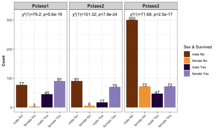
Bar Plot with Chi-square test
- The chi-square test is the kind of hypothesis test that we use to examine the relationship between two categorical variables.
barpl <- ggplot(data = plotdata) +
  geom_bar(aes(x = group, y = value, fill = group), stat = "identity", position = position_dodge()) +
  geom_text(aes(x = group, y = value, label = value), vjust = 0, color = "black", size = 4) +
  geom_text(data = test_res,
            aes(x = 4.2, y = max(plotdata$value) + 20,
                label = paste0("χ²(", parameter, ")=", round(statistic, 2), "; p=", signif(p.value, 2))),
            hjust = 1) +
  labs(x = "", y = "Count") +
  scale_fill_manual(name = "Sex & Survived",
                    values = c("#803C08", "#F1A340",
                               "#2C0a4B", "#998EC3")) +
  facet_grid(.~ Pclass, scales = "free_x") +
  theme_bw() +
  theme(axis.title.y = element_text(size = 10, face = "bold"),
        axis.text.y = element_text(size = 9),
        axis.text.x = element_text(angle = 45, hjust = 1, size = 9),
        strip.text = element_text(size = 12, face = "bold"))

barpl

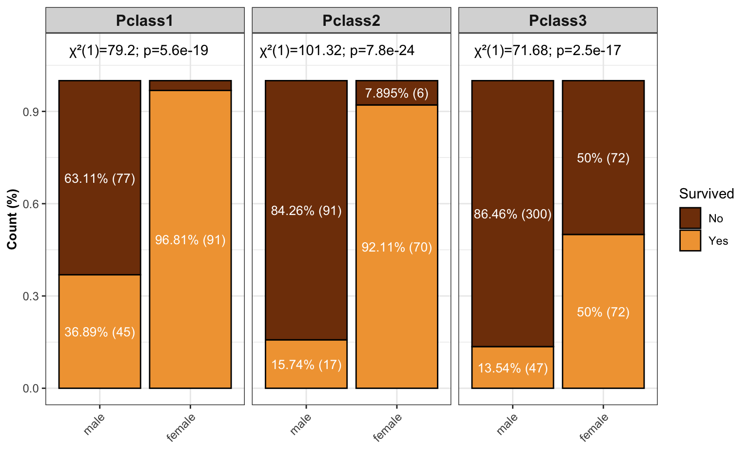
- stacked barplot
plotdata2 <- dat %>%
  dplyr::filter(Pclass == 1) %>%
  dplyr::select(PassengerId, Sex, Survived) %>%
  dplyr::group_by(Sex, Survived) %>%
  dplyr::summarise(value = n()) %>%
  dplyr::mutate(Pclass = "Pclass1") %>%
  dplyr::ungroup() %>%
  rbind(dat %>%
      dplyr::filter(Pclass == 2) %>%
      dplyr::select(PassengerId, Sex, Survived) %>%
      dplyr::group_by(Sex, Survived) %>%
      dplyr::summarise(value = n()) %>%
      dplyr::mutate(Pclass = "Pclass2") %>%
      dplyr::ungroup()
  ) %>%
  rbind(dat %>%
      dplyr::filter(Pclass == 3) %>%
      dplyr::select(PassengerId, Sex, Survived) %>%
      dplyr::group_by(Sex, Survived) %>%
      dplyr::summarise(value = n()) %>%
      dplyr::mutate(Pclass = "Pclass3") %>%
      dplyr::ungroup()
  ) %>%
  dplyr::mutate(Sex = factor(Sex, levels = c("male", "female"))) %>%
  dplyr::mutate(Survived = factor(Survived, levels = c("0", "1"), labels = c("No", "Yes"))) %>%
  dplyr::arrange(desc(Survived)) %>%
  dplyr::group_by(Pclass, Sex) %>%
  dplyr::mutate(percent = signif(value/sum(value), 4),
                pos = cumsum(percent) - 0.5*percent,
                label = paste0(percent * 100, "% (", value, ")"))


stacked_barpl <- ggplot(data = plotdata2, aes(x = Sex, y = percent)) +
  geom_bar(aes(fill = Survived),
           stat = "identity", position = "fill", color = "black") +
  geom_text(aes(label = ifelse(percent >= 0.07, label,""),
                y = pos), color = "white", size = 3.5) +
  geom_text(data = test_res,
            aes(x = 2.2, y = 1.1,
                label = paste0("χ²(", parameter, ")=", round(statistic, 2), "; p=", signif(p.value, 2))),
            hjust = 1) +
  labs(x = "", y = "Count (%)") +
  scale_fill_manual(name = "Survived",
                    values = c("#803C08", "#F1A340")) +
  # scale_y_continuous(breaks = seq(0, 1, 0.2),
  #                     labels = paste0(seq(0, 1, 0.2) * 100, "%"),
  #                     expand = expansion(mult = c(0, 0.1))) +
  facet_grid(.~ Pclass, scales = "free_x") +
  theme_bw() +
  theme(axis.title.y = element_text(size = 10, face = "bold"),
        axis.text.y = element_text(size = 9),
        axis.text.x = element_text(angle = 45, hjust = 1, size = 9),
        strip.text = element_text(size = 12, face = "bold"))

stacked_barpl
Conclusion
barplot shows the number of groups and add chi-square test into the barplot.
Systemic information
devtools::session_info()
## ─ Session info ───────────────────────────────────────────────────────────────
##  setting  value
##  version  R version 4.1.3 (2022-03-10)
##  os       macOS Big Sur/Monterey 10.16
##  system   x86_64, darwin17.0
##  ui       X11
##  language (EN)
##  collate  en_US.UTF-8
##  ctype    en_US.UTF-8
##  tz       Asia/Shanghai
##  date     2024-01-22
##  pandoc   3.1.3 @ /Users/zouhua/opt/anaconda3/bin/ (via rmarkdown)
##
## ─ Packages ───────────────────────────────────────────────────────────────────
##  package     * version date (UTC) lib source
##  blogdown      1.18    2023-06-19 [2] CRAN (R 4.1.3)
##  bookdown      0.34    2023-05-09 [2] CRAN (R 4.1.2)
##  bslib         0.6.0   2023-11-21 [1] CRAN (R 4.1.3)
##  cachem        1.0.8   2023-05-01 [2] CRAN (R 4.1.2)
##  callr         3.7.3   2022-11-02 [2] CRAN (R 4.1.2)
##  cli           3.6.1   2023-03-23 [2] CRAN (R 4.1.2)
##  colorspace    2.1-0   2023-01-23 [2] CRAN (R 4.1.2)
##  crayon        1.5.2   2022-09-29 [2] CRAN (R 4.1.2)
##  devtools      2.4.5   2022-10-11 [2] CRAN (R 4.1.2)
##  digest        0.6.33  2023-07-07 [1] CRAN (R 4.1.3)
##  dplyr       * 1.1.4   2023-11-17 [1] CRAN (R 4.1.3)
##  ellipsis      0.3.2   2021-04-29 [2] CRAN (R 4.1.0)
##  evaluate      0.21    2023-05-05 [2] CRAN (R 4.1.2)
##  fansi         1.0.4   2023-01-22 [2] CRAN (R 4.1.2)
##  farver        2.1.1   2022-07-06 [2] CRAN (R 4.1.2)
##  fastmap       1.1.1   2023-02-24 [2] CRAN (R 4.1.2)
##  forcats     * 1.0.0   2023-01-29 [1] CRAN (R 4.1.2)
##  fs            1.6.2   2023-04-25 [2] CRAN (R 4.1.2)
##  generics      0.1.3   2022-07-05 [2] CRAN (R 4.1.2)
##  ggplot2     * 3.4.4   2023-10-12 [1] CRAN (R 4.1.3)
##  glue          1.6.2   2022-02-24 [2] CRAN (R 4.1.2)
##  gtable        0.3.3   2023-03-21 [2] CRAN (R 4.1.2)
##  highr         0.10    2022-12-22 [2] CRAN (R 4.1.2)
##  hms           1.1.3   2023-03-21 [2] CRAN (R 4.1.2)
##  htmltools     0.5.7   2023-11-03 [1] CRAN (R 4.1.3)
##  htmlwidgets   1.6.2   2023-03-17 [2] CRAN (R 4.1.2)
##  httpuv        1.6.11  2023-05-11 [2] CRAN (R 4.1.3)
##  jquerylib     0.1.4   2021-04-26 [2] CRAN (R 4.1.0)
##  jsonlite      1.8.7   2023-06-29 [2] CRAN (R 4.1.3)
##  knitr         1.43    2023-05-25 [2] CRAN (R 4.1.3)
##  labeling      0.4.2   2020-10-20 [2] CRAN (R 4.1.0)
##  later         1.3.1   2023-05-02 [2] CRAN (R 4.1.2)
##  lifecycle     1.0.3   2022-10-07 [2] CRAN (R 4.1.2)
##  lubridate   * 1.9.2   2023-02-10 [2] CRAN (R 4.1.2)
##  magrittr      2.0.3   2022-03-30 [2] CRAN (R 4.1.2)
##  memoise       2.0.1   2021-11-26 [2] CRAN (R 4.1.0)
##  mime          0.12    2021-09-28 [2] CRAN (R 4.1.0)
##  miniUI        0.1.1.1 2018-05-18 [2] CRAN (R 4.1.0)
##  munsell       0.5.0   2018-06-12 [2] CRAN (R 4.1.0)
##  pillar        1.9.0   2023-03-22 [2] CRAN (R 4.1.2)
##  pkgbuild      1.4.2   2023-06-26 [2] CRAN (R 4.1.3)
##  pkgconfig     2.0.3   2019-09-22 [2] CRAN (R 4.1.0)
##  pkgload       1.3.2.1 2023-07-08 [2] CRAN (R 4.1.3)
##  prettyunits   1.1.1   2020-01-24 [2] CRAN (R 4.1.0)
##  processx      3.8.2   2023-06-30 [2] CRAN (R 4.1.3)
##  profvis       0.3.8   2023-05-02 [2] CRAN (R 4.1.2)
##  promises      1.2.0.1 2021-02-11 [2] CRAN (R 4.1.0)
##  ps            1.7.5   2023-04-18 [2] CRAN (R 4.1.2)
##  purrr       * 1.0.1   2023-01-10 [1] CRAN (R 4.1.2)
##  R6            2.5.1   2021-08-19 [2] CRAN (R 4.1.0)
##  Rcpp          1.0.11  2023-07-06 [1] CRAN (R 4.1.3)
##  readr       * 2.1.4   2023-02-10 [1] CRAN (R 4.1.2)
##  remotes       2.4.2   2021-11-30 [2] CRAN (R 4.1.0)
##  rlang         1.1.1   2023-04-28 [1] CRAN (R 4.1.2)
##  rmarkdown     2.23    2023-07-01 [2] CRAN (R 4.1.3)
##  rstudioapi    0.15.0  2023-07-07 [2] CRAN (R 4.1.3)
##  sass          0.4.6   2023-05-03 [2] CRAN (R 4.1.2)
##  scales        1.2.1   2022-08-20 [1] CRAN (R 4.1.2)
##  sessioninfo   1.2.2   2021-12-06 [2] CRAN (R 4.1.0)
##  shiny         1.7.4.1 2023-07-06 [2] CRAN (R 4.1.3)
##  stringi       1.7.12  2023-01-11 [2] CRAN (R 4.1.2)
##  stringr     * 1.5.1   2023-11-14 [1] CRAN (R 4.1.3)
##  tibble      * 3.2.1   2023-03-20 [1] CRAN (R 4.1.2)
##  tidyr       * 1.3.0   2023-01-24 [1] CRAN (R 4.1.2)
##  tidyselect    1.2.0   2022-10-10 [2] CRAN (R 4.1.2)
##  tidyverse   * 2.0.0   2023-02-22 [1] CRAN (R 4.1.2)
##  timechange    0.2.0   2023-01-11 [2] CRAN (R 4.1.2)
##  titanic     * 0.1.0   2015-08-31 [1] CRAN (R 4.1.0)
##  tzdb          0.4.0   2023-05-12 [2] CRAN (R 4.1.3)
##  urlchecker    1.0.1   2021-11-30 [2] CRAN (R 4.1.0)
##  usethis       2.2.2   2023-07-06 [2] CRAN (R 4.1.3)
##  utf8          1.2.3   2023-01-31 [2] CRAN (R 4.1.2)
##  vctrs         0.6.5   2023-12-01 [1] CRAN (R 4.1.3)
##  withr         2.5.0   2022-03-03 [2] CRAN (R 4.1.2)
##  xfun          0.40    2023-08-09 [1] CRAN (R 4.1.3)
##  xtable        1.8-4   2019-04-21 [2] CRAN (R 4.1.0)
##  yaml          2.3.7   2023-01-23 [2] CRAN (R 4.1.2)
##
##  [1] /Users/zouhua/Library/R/x86_64/4.1/library
##  [2] /Library/Frameworks/R.framework/Versions/4.1/Resources/library
##
## ──────────────────────────────────────────────────────────────────────────────
Hua Zou
Senior Bioinformatic Analyst
My research interests include host-microbiota intersection, machine learning and multi-omics data integration.