R visualization: scatter plot on PCA by ggplot2
scatter plot on PCA
Introduction
Display the results of PCA (Principle Components Analysis) by using a scatterplot. It’s also necessary to draw the boundaries of the group. Here, this tutorial would give four approaches to do this using ggplot2.
Loading required packages
knitr::opts_chunk$set(message = FALSE, warning = FALSE)

library(tidyverse)
library(patchwork)

# rm(list = ls())
options(stringsAsFactors = F)

# group & color
group_names <- c("A", "B", "C")
group_colors <- c("#0073C2FF", "#EFC000FF", "#CD534CFF")
group_shapes <- c(15, 16, 17)
Data preparation
- Constructing data object
dat <- data.frame(
  SampleID = paste0("S_", 1:24),
  PC1 = c(0.022770707, 0.054692482, 0.039981067, 0.007793265, 7.84e-06, -0.009869502, -0.059123147,
          -0.100341862, 0.027247694, 0.156717826, 0.247041497, 0.181258984, 0.172786176,
          0.131875865, 0.230052533, 0.163389878, -0.116222295, -0.221050628, -0.084606354,
          -0.214705258, -0.210235971, -0.200839043, -0.06763774, -0.175523677),
  PC2 = c(-0.05555032, -0.050592178, -0.070996307, -0.037754744, -0.091904909, -0.067078552,
          -0.114239498, -0.099288661, 0.024239885, 0.06885023, 0.005302438, 0.035700696, 0.042451004,
          0.019859585, 0.019250596, 0.031094568, 0.022300445, 0.057798633, 0.08757355, 0.048752276,
          0.021344081, 0.055314429, -0.005297042, 0.10518067),
  PC3 = c(-0.052194396, 0.000958851, 0.006141922, 0.048682841, -0.061645805, -0.003102679, 0.028396414,
          0.01980974, -0.055276428, -0.082034627, 0.081183975, 0.030190352, -0.035916706, -0.052318759,
          0.016482896, 0.096296503, -0.01270539, 0.019406331, 0.033471156, 0.003175988, 0.020986428,
          0.025259074, -0.093440324, 0.062841498),
  Group = c(rep("A", 8), rep("B", 8), rep("C", 8)),
  PID = paste0("P", rep(1:8, 3)))
Notice:
SampleID: sample names
PC1: the first principle component from PCA
PC2: the second principle component from PCA
PC3: the third principle component from PCA
Group: group information
PID: participant identity
- Factorizing Group
plotdata <- dat |>
  dplyr::mutate(Group = factor(Group, levels = group_names))

head(plotdata)
##   SampleID          PC1         PC2          PC3 Group PID
## 1      S_1  0.022770707 -0.05555032 -0.052194396     A  P1
## 2      S_2  0.054692482 -0.05059218  0.000958851     A  P2
## 3      S_3  0.039981067 -0.07099631  0.006141922     A  P3
## 4      S_4  0.007793265 -0.03775474  0.048682841     A  P4
## 5      S_5  0.000007840 -0.09190491 -0.061645805     A  P5
## 6      S_6 -0.009869502 -0.06707855 -0.003102679     A  P6
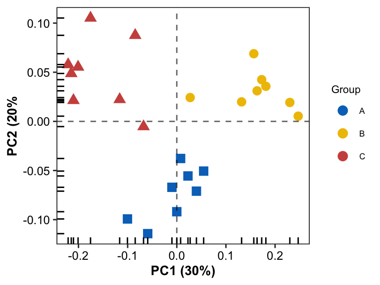
Simple Scatter Plot
- create poing by
geom_point
pl0 <- ggplot(data = plotdata, aes(x = PC1, y = PC2)) +
  geom_point(aes(color = Group, shape = Group), size = 3) +
  geom_rug() +
  geom_hline(yintercept = 0, linetype = 2, linewidth = 0.5, alpha = 0.6) +
  geom_vline(xintercept = 0, linetype = 2, linewidth = 0.5, alpha = 0.6) +
  labs(x = "PC1 (30%)", y = "PC2 (20%") +
  scale_color_manual(values = group_colors) +
  scale_shape_manual(values = group_shapes) +
  guides(shape = "none") +
  theme_bw() +
  theme(plot.title = element_text(size = 10, color = "black", face = "bold", hjust = 0.5),
        axis.title = element_text(size = 10, color = "black", face = "bold"),
        axis.text = element_text(size = 9, color = "black"),
        text = element_text(size = 8, color = "black"),
        strip.text = element_text(size = 9, color = "black", face = "bold"),
        panel.grid = element_blank(),
        panel.background = element_rect(color = "black", fill = "transparent"),
        legend.key = element_rect(fill = "transparent"))

pl0
Scatter Plot with confidence interval of group
- add confidence interval ellipse by
stat_ellipse
pl1 <-  pl0 + stat_ellipse(aes(color = Group), level = 0.95, linetype = 1, show.legend = FALSE)

pl1
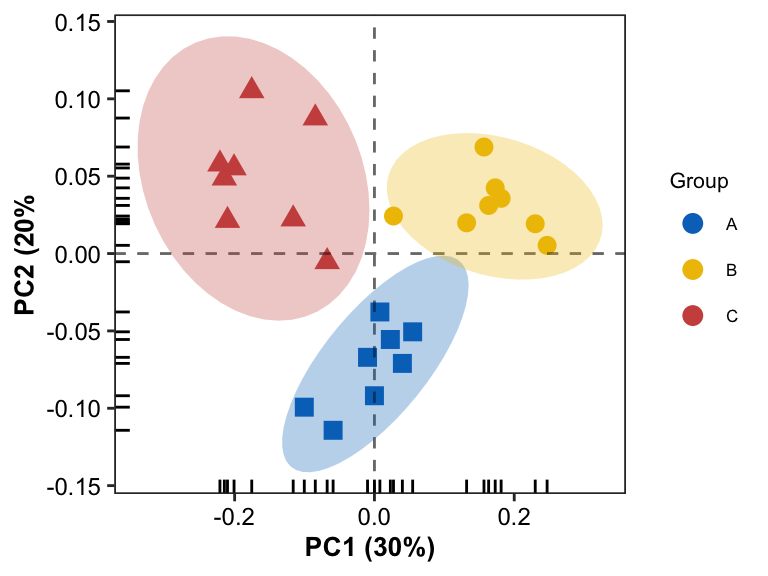
Another Scatter Plot with confidence interval
- add confidence interval ellipse by
stat_ellipse
pl2 <-  pl0 + stat_ellipse(aes(fill = Group), geom = "polygon", level = 0.95, alpha = 0.3, show.legend = FALSE) +
    scale_fill_manual(values = group_colors)

pl2
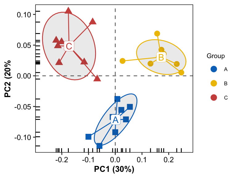
Scatter Plot with enterotype
- Add enterotype by
geom_enterotype
# https://github.com/cran/miscTools/
insertRow <- function(m, r, v = NA, rName = "") {

  if (!inherits(m, "matrix")) {
    stop("argument 'm' must be a matrix")
  }
  if (r == as.integer(r)) {
    r <- as.integer(r)
  }
  else {
    stop("argument 'r' must be an integer")
  }
  if (length(r) != 1) {
    stop("argument 'r' must be a scalar")
  }
  if (r < 1) {
    stop("argument 'r' must be positive")
  }
  if (r > nrow(m) + 1) {
    stop("argument 'r' must not be larger than the number of rows",
         " of matrix 'm' plus one")
  }
  if (!is.character(rName)) {
    stop("argument 'rName' must be a character string")
  }
  if (length(rName) != 1) {
    stop("argument 'rName' must be a be a single character string")
  }
  nr <- nrow(m)
  nc <- ncol(m)
  rNames <- rownames(m)
  if (is.null(rNames) & rName != "") {
    rNames <- rep("", nr)
  }
  if (r == 1) {
    m2 <- rbind(matrix(v, ncol = nc), m)
    if (!is.null(rNames)) {
      rownames(m2) <- c(rName, rNames)
    }
  }
  else if (r == nr + 1) {
    m2 <- rbind(m, matrix(v, ncol = nc))
    if (!is.null(rNames)) {
      rownames(m2) <- c(rNames, rName)
    }
  }
  else {
    m2 <- rbind(m[1:(r - 1), , drop = FALSE], matrix(v, ncol = nc),
                m[r:nr, , drop = FALSE])
    if (!is.null(rNames)) {
      rownames(m2) <- c(rNames[1:(r - 1)], rName, rNames[r:nr])
    }
  }
  return(m2)
}


# https://stackoverflow.com/questions/42575769/how-to-modify-the-backgroup-color-of-label-in-the-multiple-ggproto-using-ggplot2
geom_enterotype <- function(
    mapping = NULL,
    data = NULL,
    stat = "identity",
    position = "identity",
    alpha = 0.2,
    prop = 0.5,
    lineend = "butt",
    linejoin = "round",
    linemitre = 1,
    arrow = NULL,
    na.rm = FALSE,
    parse = FALSE,
    nudge_x = 0,
    nudge_y = 0,
    label.padding = unit(0.15, "lines"),
    label.r = unit(0.15, "lines"),
    label.size = 0.1,
    show.legend = TRUE,
    inherit.aes = TRUE,
    ...) {

  # create new stat and geom for scatterplot with ellipses
  StatEllipse <- ggproto(
    "StatEllipse",
    Stat,
    required_aes = c("x", "y"),
    compute_group = function(., data, scales, level = 0.75, segments = 51, ...) {
        #library(MASS)
        dfn <- 2
        dfd <- length(data$x) - 1
        if (dfd < 3) {
           ellipse <- rbind(c(NA, NA))
        } else {
          v <- MASS::cov.trob(cbind(data$x, data$y))
          shape <- v$cov
          center <- v$center
          radius <- sqrt(dfn * qf(level, dfn, dfd))
          angles <- (0:segments) * 2 * pi / segments
          unit.circle <- cbind(cos(angles), sin(angles))
          ellipse <- t(center + radius * t(unit.circle %*% chol(shape)))
        }
        ellipse <- as.data.frame(ellipse)
        colnames(ellipse) <- c("x", "y")

        return(ellipse)
      }
  )

  # write new ggproto
  GeomEllipse <- ggproto(
    "GeomEllipse",
    Geom,
    draw_group = function(data, panel_scales, coord) {
        n <- nrow(data)
        if (n == 1) {
          return(zeroGrob())
        }
        munched <- coord_munch(coord, data, panel_scales)
        munched <- munched[order(munched$group), ]
        first_idx <- !duplicated(munched$group)
        first_rows <- munched[first_idx, ]
        grid::pathGrob(munched$x, munched$y, default.units = "native",
                       id = munched$group,
                       gp = grid::gpar(col = first_rows$colour,
                                       fill = alpha(first_rows$fill, first_rows$alpha),
                                       lwd = first_rows$size * .pt,
                                       lty = first_rows$linetype))
        }, default_aes = aes(colour = "NA", fill = "grey20", size = 0.5,
                             linetype = 1, alpha = NA, prop = 0.5),
          handle_na = function(data, params) {data},
          required_aes = c("x", "y"),
          draw_key = draw_key_path
  )

  # create a new stat for PCA scatterplot with lines which totally directs to the center
  StatConline <- ggproto(
    "StatConline",
    Stat,
    compute_group = function(data, scales) {
        df <- data.frame(data$x, data$y)
        mat <- as.matrix(df)
        center <- MASS::cov.trob(df)$center
        names(center) <- NULL
        mat_insert <- insertRow(mat, 2, center)
        for(i in 1:nrow(mat)) {
            mat_insert <- insertRow(mat_insert, 2*i, center)
            next
        }
        mat_insert <- mat_insert[-c(2:3), ]
        rownames(mat_insert) <- NULL
        mat_insert <- as.data.frame(mat_insert, center)
        colnames(mat_insert) <- c("x", "y")
        return(mat_insert)
      }, required_aes = c("x", "y")
  )

  # create a new stat for PCA scatterplot with center labels
  StatLabel <- ggproto(
    "StatLabel",
    Stat,
    compute_group = function(data, scales) {
        df <- data.frame(data$x, data$y)
        center <- MASS::cov.trob(df)$center
        names(center) <- NULL
        center <- t(as.data.frame(center))
        center <- as.data.frame(cbind(center))
        colnames(center) <- c("x", "y")
        rownames(center) <- NULL
        return(center)
       }, required_aes = c("x", "y")
  )

  layer1 <- layer(data = data,
                  mapping = mapping,
                  stat = stat,
                  geom = GeomPoint,
                  position = position,
                  show.legend = show.legend,
                  inherit.aes = inherit.aes,
                  params = list(na.rm = na.rm, ...))

  layer2 <- layer(data = data,
                  mapping = mapping,
                  stat = StatEllipse,
                  geom = GeomEllipse,
                  position = position,
                  show.legend = FALSE,
                  inherit.aes = inherit.aes,
                  params = list(na.rm = na.rm, prop = prop, alpha = alpha, ...))

  layer3 <- layer(data = data,
                  mapping = mapping,
                  stat = StatConline,
                  geom = GeomPath,
                  position = position,
                  show.legend = show.legend,
                  inherit.aes = inherit.aes,
                  params = list(lineend = lineend, linejoin = linejoin,
                                linemitre = linemitre, arrow = arrow, na.rm = na.rm, ...))

  if (!missing(nudge_x) || !missing(nudge_y)) {
    if (!missing(position)) {
      stop("Specify either `position` or `nudge_x`/`nudge_y`",
           call. = FALSE)
    }
    position <- position_nudge(nudge_x, nudge_y)
  }
  layer4 <- layer(data = data,
                  mapping = mapping,
                  stat = StatLabel,
                  geom = GeomLabel,
                  position = position,
                  show.legend = FALSE,
                  inherit.aes = inherit.aes,
                  params = list(parse = parse, label.padding = label.padding,
                                label.r = label.r, label.size = label.size, na.rm = na.rm, ...))

  return(list(layer1, layer2, layer3, layer4))
}
- plotting
pl3 <- pl0 + geom_enterotype(aes(color = Group, label = Group), show.legend = FALSE, alpha = 0.1)

pl3
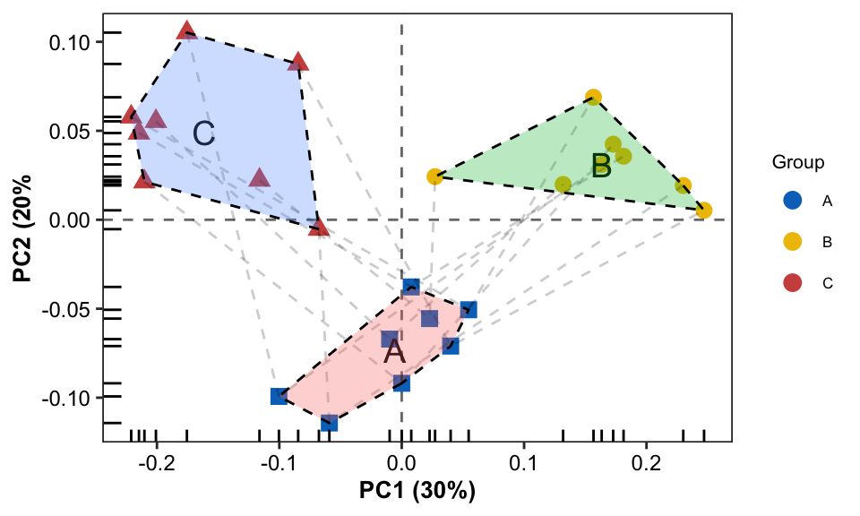
Scatter Plot with the border line
Calculating the position of group label
Calculating the position of outlier per group
Compvar_position <- cbind(PC1 = tapply(plotdata$PC1, plotdata$Group, mean),
                          PC2 = tapply(plotdata$PC2, plotdata$Group, mean)) %>%
  as.data.frame() %>%
  tibble::rownames_to_column("Group")

border_fun <- function(x = plotdata, grp) {

  tempdat <- x[x$Group %in% grp, , F]
  res <- tempdat[chull(tempdat[[2]], tempdat[[3]]), ]

  return(res)
}

Compvar_border <- NULL
for (i in 1:length(unique(plotdata$Group))) {
  Compvar_border <- rbind(Compvar_border, border_fun(grp = unique(plotdata$Group)[i]))
}
- Plotting
pl4 <- pl0 + geom_line(aes(group = PID), linetype = 2, alpha = 0.2) +
  geom_text(data = Compvar_position, aes(x = PC1, y = PC2, label = Group), show.legend = FALSE, size = 5) +
  geom_polygon(data = Compvar_border, aes(fill = Group), color = "black", alpha = 0.3, linetype = 2, show.legend = FALSE) +
  scale_color_manual(values = group_colors)

pl4
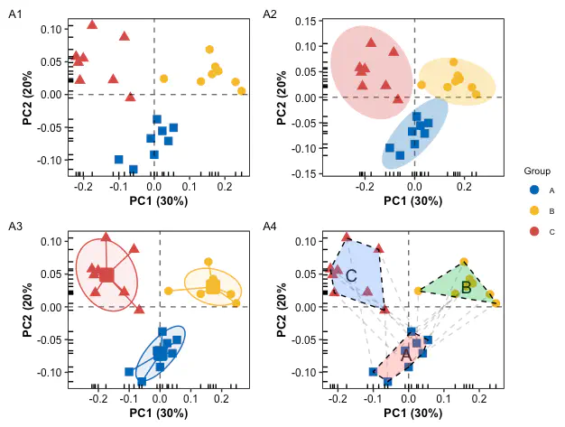
Combination
pl0 + pl1 + pl3 + pl4 + plot_layout(ncol = 2, guides = "collect") +
  plot_annotation(tag_levels = c(1), tag_prefix = "A")
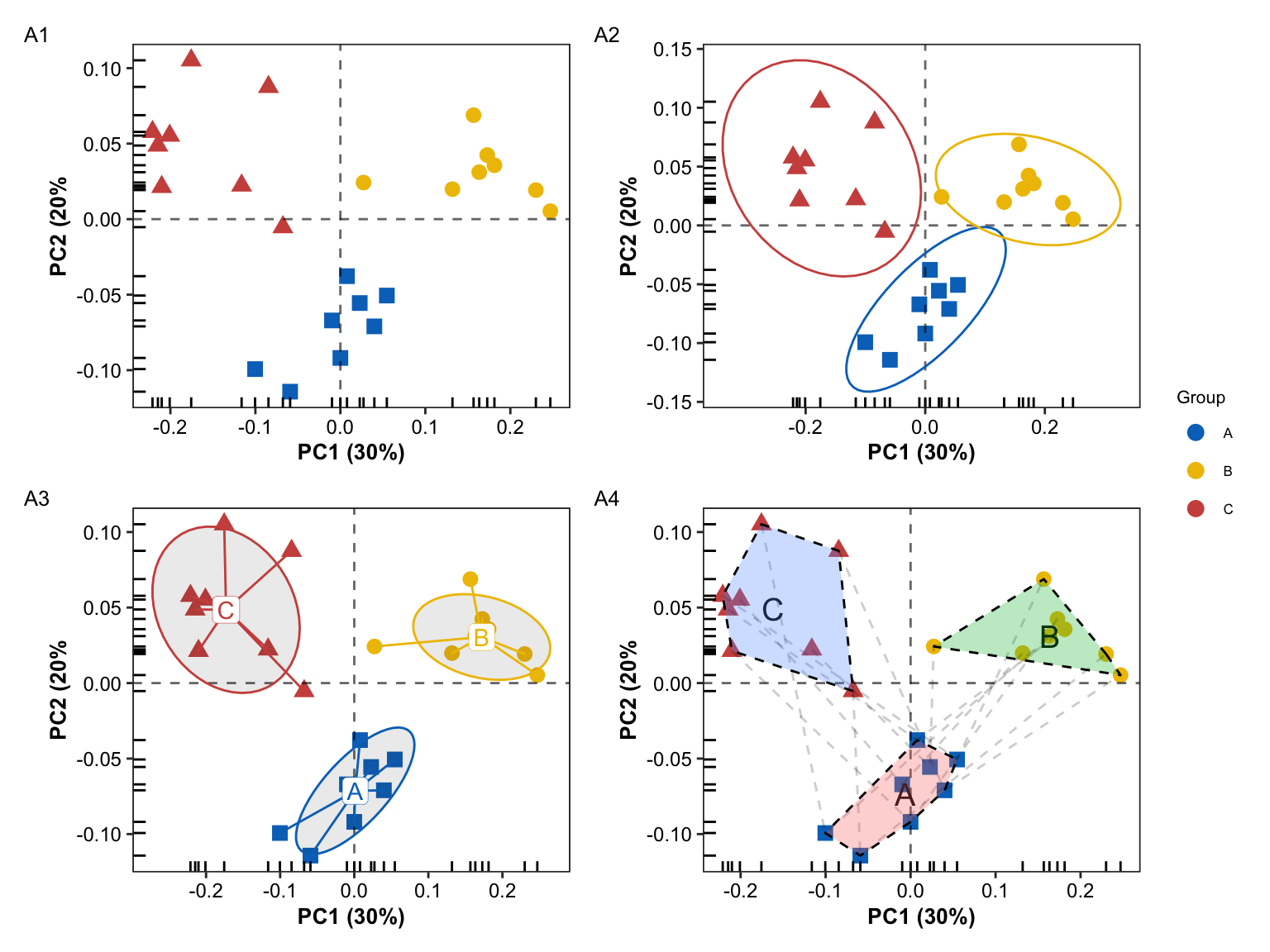
Conclusion
Compared to the single PCA scatterplot, the scatterplot with the addition of the group boundary can more directly reflect the difference information between groups.
Systemic information
devtools::session_info()
## ─ Session info ───────────────────────────────────────────────────────────────
##  setting  value
##  version  R version 4.1.3 (2022-03-10)
##  os       macOS Big Sur/Monterey 10.16
##  system   x86_64, darwin17.0
##  ui       X11
##  language (EN)
##  collate  en_US.UTF-8
##  ctype    en_US.UTF-8
##  tz       Asia/Shanghai
##  date     2023-08-05
##  pandoc   3.1.3 @ /Users/zouhua/opt/anaconda3/bin/ (via rmarkdown)
##
## ─ Packages ───────────────────────────────────────────────────────────────────
##  package     * version date (UTC) lib source
##  blogdown      1.18    2023-06-19 [2] CRAN (R 4.1.3)
##  bookdown      0.34    2023-05-09 [2] CRAN (R 4.1.2)
##  bslib         0.5.0   2023-06-09 [2] CRAN (R 4.1.3)
##  cachem        1.0.8   2023-05-01 [2] CRAN (R 4.1.2)
##  callr         3.7.3   2022-11-02 [2] CRAN (R 4.1.2)
##  cli           3.6.1   2023-03-23 [2] CRAN (R 4.1.2)
##  colorspace    2.1-0   2023-01-23 [2] CRAN (R 4.1.2)
##  crayon        1.5.2   2022-09-29 [2] CRAN (R 4.1.2)
##  devtools      2.4.5   2022-10-11 [2] CRAN (R 4.1.2)
##  digest        0.6.33  2023-07-07 [1] CRAN (R 4.1.3)
##  dplyr       * 1.1.2   2023-04-20 [2] CRAN (R 4.1.2)
##  ellipsis      0.3.2   2021-04-29 [2] CRAN (R 4.1.0)
##  evaluate      0.21    2023-05-05 [2] CRAN (R 4.1.2)
##  fansi         1.0.4   2023-01-22 [2] CRAN (R 4.1.2)
##  farver        2.1.1   2022-07-06 [2] CRAN (R 4.1.2)
##  fastmap       1.1.1   2023-02-24 [2] CRAN (R 4.1.2)
##  forcats     * 1.0.0   2023-01-29 [2] CRAN (R 4.1.2)
##  fs            1.6.2   2023-04-25 [2] CRAN (R 4.1.2)
##  generics      0.1.3   2022-07-05 [2] CRAN (R 4.1.2)
##  ggplot2     * 3.4.2   2023-04-03 [2] CRAN (R 4.1.2)
##  glue          1.6.2   2022-02-24 [2] CRAN (R 4.1.2)
##  gtable        0.3.3   2023-03-21 [2] CRAN (R 4.1.2)
##  highr         0.10    2022-12-22 [2] CRAN (R 4.1.2)
##  hms           1.1.3   2023-03-21 [2] CRAN (R 4.1.2)
##  htmltools     0.5.5   2023-03-23 [2] CRAN (R 4.1.2)
##  htmlwidgets   1.6.2   2023-03-17 [2] CRAN (R 4.1.2)
##  httpuv        1.6.11  2023-05-11 [2] CRAN (R 4.1.3)
##  jquerylib     0.1.4   2021-04-26 [2] CRAN (R 4.1.0)
##  jsonlite      1.8.7   2023-06-29 [2] CRAN (R 4.1.3)
##  knitr         1.43    2023-05-25 [2] CRAN (R 4.1.3)
##  labeling      0.4.2   2020-10-20 [2] CRAN (R 4.1.0)
##  later         1.3.1   2023-05-02 [2] CRAN (R 4.1.2)
##  lifecycle     1.0.3   2022-10-07 [2] CRAN (R 4.1.2)
##  lubridate   * 1.9.2   2023-02-10 [2] CRAN (R 4.1.2)
##  magrittr      2.0.3   2022-03-30 [2] CRAN (R 4.1.2)
##  MASS          7.3-60  2023-05-04 [2] CRAN (R 4.1.2)
##  memoise       2.0.1   2021-11-26 [2] CRAN (R 4.1.0)
##  mime          0.12    2021-09-28 [2] CRAN (R 4.1.0)
##  miniUI        0.1.1.1 2018-05-18 [2] CRAN (R 4.1.0)
##  munsell       0.5.0   2018-06-12 [2] CRAN (R 4.1.0)
##  patchwork   * 1.1.2   2022-08-19 [2] CRAN (R 4.1.2)
##  pillar        1.9.0   2023-03-22 [2] CRAN (R 4.1.2)
##  pkgbuild      1.4.2   2023-06-26 [2] CRAN (R 4.1.3)
##  pkgconfig     2.0.3   2019-09-22 [2] CRAN (R 4.1.0)
##  pkgload       1.3.2.1 2023-07-08 [2] CRAN (R 4.1.3)
##  prettyunits   1.1.1   2020-01-24 [2] CRAN (R 4.1.0)
##  processx      3.8.2   2023-06-30 [2] CRAN (R 4.1.3)
##  profvis       0.3.8   2023-05-02 [2] CRAN (R 4.1.2)
##  promises      1.2.0.1 2021-02-11 [2] CRAN (R 4.1.0)
##  ps            1.7.5   2023-04-18 [2] CRAN (R 4.1.2)
##  purrr       * 1.0.1   2023-01-10 [2] CRAN (R 4.1.2)
##  R6            2.5.1   2021-08-19 [2] CRAN (R 4.1.0)
##  Rcpp          1.0.11  2023-07-06 [1] CRAN (R 4.1.3)
##  readr       * 2.1.4   2023-02-10 [2] CRAN (R 4.1.2)
##  remotes       2.4.2   2021-11-30 [2] CRAN (R 4.1.0)
##  rlang         1.1.1   2023-04-28 [2] CRAN (R 4.1.2)
##  rmarkdown     2.23    2023-07-01 [2] CRAN (R 4.1.3)
##  rstudioapi    0.15.0  2023-07-07 [2] CRAN (R 4.1.3)
##  sass          0.4.6   2023-05-03 [2] CRAN (R 4.1.2)
##  scales        1.2.1   2022-08-20 [2] CRAN (R 4.1.2)
##  sessioninfo   1.2.2   2021-12-06 [2] CRAN (R 4.1.0)
##  shiny         1.7.4.1 2023-07-06 [2] CRAN (R 4.1.3)
##  stringi       1.7.12  2023-01-11 [2] CRAN (R 4.1.2)
##  stringr     * 1.5.0   2022-12-02 [2] CRAN (R 4.1.2)
##  tibble      * 3.2.1   2023-03-20 [2] CRAN (R 4.1.2)
##  tidyr       * 1.3.0   2023-01-24 [2] CRAN (R 4.1.2)
##  tidyselect    1.2.0   2022-10-10 [2] CRAN (R 4.1.2)
##  tidyverse   * 2.0.0   2023-02-22 [1] CRAN (R 4.1.2)
##  timechange    0.2.0   2023-01-11 [2] CRAN (R 4.1.2)
##  tzdb          0.4.0   2023-05-12 [2] CRAN (R 4.1.3)
##  urlchecker    1.0.1   2021-11-30 [2] CRAN (R 4.1.0)
##  usethis       2.2.2   2023-07-06 [2] CRAN (R 4.1.3)
##  utf8          1.2.3   2023-01-31 [2] CRAN (R 4.1.2)
##  vctrs         0.6.3   2023-06-14 [1] CRAN (R 4.1.3)
##  withr         2.5.0   2022-03-03 [2] CRAN (R 4.1.2)
##  xfun          0.39    2023-04-20 [2] CRAN (R 4.1.2)
##  xtable        1.8-4   2019-04-21 [2] CRAN (R 4.1.0)
##  yaml          2.3.7   2023-01-23 [2] CRAN (R 4.1.2)
##
##  [1] /Users/zouhua/Library/R/x86_64/4.1/library
##  [2] /Library/Frameworks/R.framework/Versions/4.1/Resources/library
##
## ──────────────────────────────────────────────────────────────────────────────
Hua Zou
Senior Bioinformatic Analyst
My research interests include host-microbiota intersection, machine learning and multi-omics data integration.