R visualization: STAMP by ggplot2
STAMP with barplot and error bar plot
Introduction
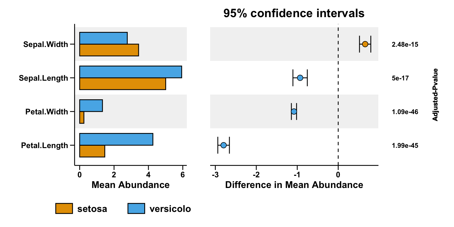
STAMP shows the mean abundance/value/proportion of features and the statistical results (t-test or wilcox-test) between groups.
Loading required packages
knitr::opts_chunk$set(message = FALSE, warning = FALSE)

library(tidyverse)
library(broom)
library(patchwork)

rm(list = ls())
options(stringsAsFactors = F)

group_names <- c("setosa", "versicolor")
group_colors <- c("#E69F00", "#56B4E9")
Data preparation for hypothesis testing
Loading iris dataset
Factorizing Species
data("iris")

test_data <- iris |>
  dplyr::select(Species, Sepal.Length, Sepal.Width, Petal.Length, Petal.Width) |>
  dplyr::filter(Species %in% group_names) |>
  dplyr::mutate(Species = factor(Species, levels = group_names))

head(test_data)
##   Species Sepal.Length Sepal.Width Petal.Length Petal.Width
## 1  setosa          5.1         3.5          1.4         0.2
## 2  setosa          4.9         3.0          1.4         0.2
## 3  setosa          4.7         3.2          1.3         0.2
## 4  setosa          4.6         3.1          1.5         0.2
## 5  setosa          5.0         3.6          1.4         0.2
## 6  setosa          5.4         3.9          1.7         0.4
- T-test for normal distribution, otherwise wilcox’s test
test_res <- test_data %>%
  dplyr::select_if(is.numeric) %>%
  purrr::map_df(~ broom::tidy(t.test(. ~ Species, data = test_data)), .id = 'Vars') |>
  dplyr::mutate(adjustP = p.adjust(p.value, method = "BH")) |>
  dplyr::filter(adjustP < 0.05)

# test_res <- test_data %>%
#   dplyr::select_if(is.numeric) %>%
#   purrr::map_df(~ broom::tidy(wilcox.test(. ~ Species, data = test_data)), .id = 'Vars') |>
#   dplyr::mutate(adjustP = p.adjust(p.value, method = "BH")) |>
#   dplyr::filter(adjustP < 0.05)

head(test_res)
## # A tibble: 4 × 12
##   Vars        estimate estimate1 estimate2 statistic  p.value parameter conf.low
##   <chr>          <dbl>     <dbl>     <dbl>     <dbl>    <dbl>     <dbl>    <dbl>
## 1 Sepal.Leng…   -0.93      5.01       5.94    -10.5  3.75e-17      86.5   -1.11
## 2 Sepal.Width    0.658     3.43       2.77      9.45 2.48e-15      94.7    0.520
## 3 Petal.Leng…   -2.80      1.46       4.26    -39.5  9.93e-46      62.1   -2.94
## 4 Petal.Width   -1.08      0.246      1.33    -34.1  2.72e-47      74.8   -1.14
## # ℹ 4 more variables: conf.high <dbl>, method <chr>, alternative <chr>,
## #   adjustP <dbl>
Data preparation for plotting
- data for left subfigure, which is barplot
data_left <- test_data |>
  dplyr::select(all_of(c("Species", test_res$Vars))) |>
  tidyr::pivot_longer(cols = -Species,
                      names_to = "Variables",
                      values_to = "Values") |>
  dplyr::group_by(Variables, Species) %>%
  dplyr::summarise(Mean = mean(Values), .groups = "drop")

head(data_left)
## # A tibble: 6 × 3
##   Variables    Species     Mean
##   <chr>        <fct>      <dbl>
## 1 Petal.Length setosa     1.46
## 2 Petal.Length versicolor 4.26
## 3 Petal.Width  setosa     0.246
## 4 Petal.Width  versicolor 1.33
## 5 Sepal.Length setosa     5.01
## 6 Sepal.Length versicolor 5.94
- data for right subfigure, which is error bar plot
data_right <- test_res |>
  dplyr::select(Vars, estimate, conf.low, conf.high, p.value, adjustP) |>
  dplyr::mutate(Species = ifelse(estimate > 0, group_names[1], group_names[2])) |>
  dplyr::arrange(desc(estimate)) |>
  dplyr::mutate(p.value = signif(p.value, 3),
                adjustP = signif(adjustP, 3)) |>
  dplyr::mutate(p.value = as.character(p.value),
                adjustP = as.character(adjustP))

head(data_right)
## # A tibble: 4 × 7
##   Vars         estimate conf.low conf.high p.value  adjustP  Species
##   <chr>           <dbl>    <dbl>     <dbl> <chr>    <chr>    <chr>
## 1 Sepal.Width     0.658    0.520     0.796 2.48e-15 2.48e-15 setosa
## 2 Sepal.Length   -0.93    -1.11     -0.754 3.75e-17 5e-17    versicolor
## 3 Petal.Width    -1.08    -1.14     -1.02  2.72e-47 1.09e-46 versicolor
## 4 Petal.Length   -2.80    -2.94     -2.66  9.93e-46 1.99e-45 versicolor
- Order variables in two dataset
data_left$Variables <- factor(data_left$Variables, levels = rev(data_right$Vars))

data_right$Vars <- factor(data_right$Vars, levels = levels(data_left$Variables))
Plotting
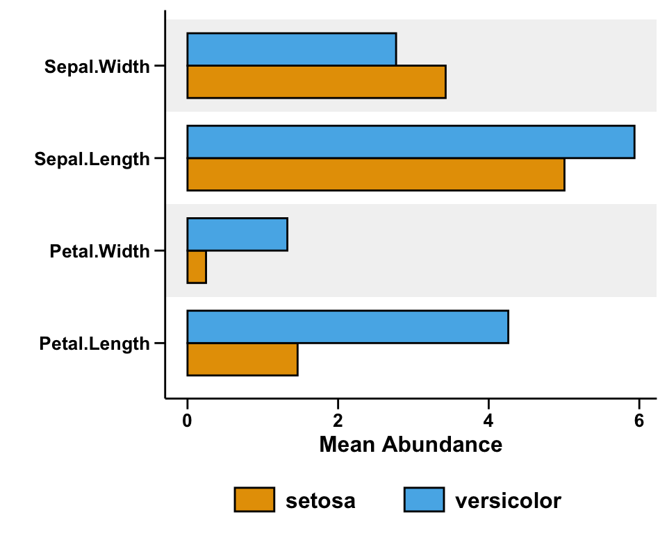
left subfigure
apply
geom_barfor barplotadd segement by
annotate
pl_left_bar <- ggplot(data_left, aes(x = Variables, y = Mean, fill = Species)) +
    scale_x_discrete(limits = levels(data_left$Variables)) +
    coord_flip() +
    labs(x = "", y = "Mean Abundance") +
    theme(panel.background = element_rect(fill = "transparent"),
          panel.grid = element_blank(),
          axis.ticks.length = unit(0.4, "lines"),
          axis.ticks = element_line(color = "black"),
          axis.line = element_line(color = "black"),
          axis.title.x = element_text(color = "black", size = 12, face = "bold"),
          axis.text = element_text(color = "black", size = 10, face = "bold"),
          legend.title = element_blank(),
          legend.text = element_text(size = 12, face = "bold",
                                     color = "black", margin = margin(r = 20)),
          legend.position = "bottom",
          legend.direction = "horizontal",
          legend.key.width = unit(0.8, "cm"),
          legend.key.height = unit(0.5, "cm"))

for (i in 1:(nrow(data_right) - 1)) {
    pl_left_bar <- pl_left_bar + annotate("rect", xmin = i + 0.5, xmax = i+1.5, ymin = -Inf, ymax = Inf,
                        fill = ifelse(i %% 2 == 0, 'white', 'gray95'))
}

pl_left_bar <- pl_left_bar +
    geom_bar(stat = "identity", position = "dodge", width = 0.7, color = "black") +
    scale_fill_manual(values = group_colors)

pl_left_bar
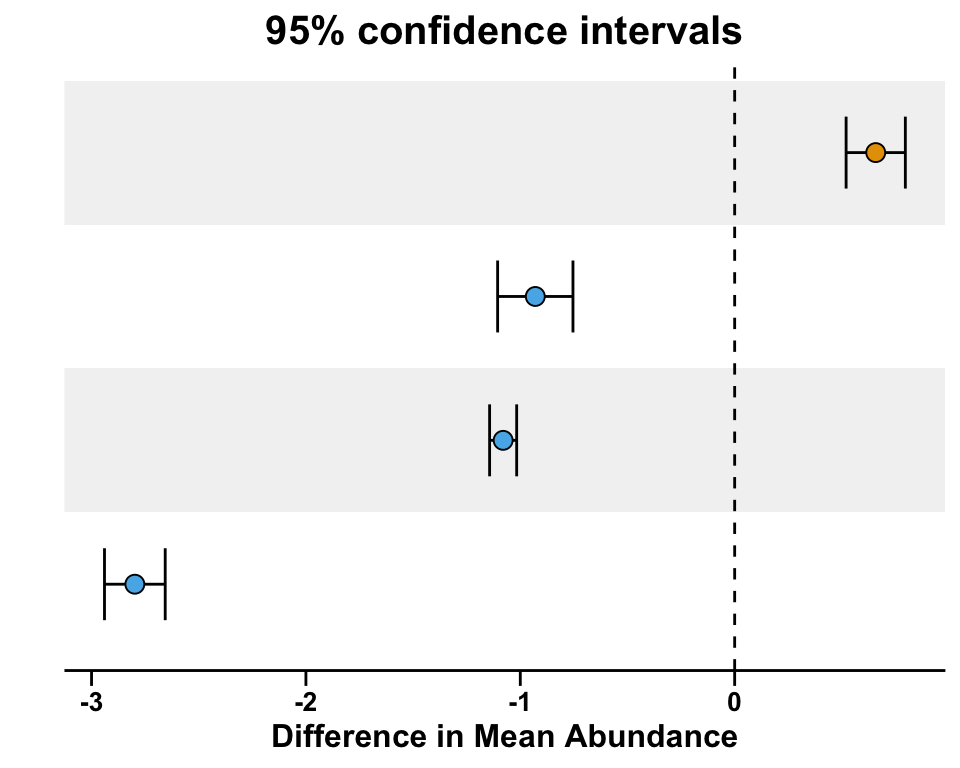
right subfigure for error bar
apply
geom_errorbarfor error baradd segement by
annotate
pl_right_scatter <- ggplot(data_right, aes(x = Vars, y = estimate, fill = Species)) +
    theme(panel.background = element_rect(fill = 'transparent'),
          panel.grid = element_blank(),
          axis.ticks.length = unit(0.4, "lines"),
          axis.ticks = element_line(color = "black"),
          axis.line = element_line(color = "black"),
          axis.title.x = element_text(color = "black", size = 12,face = "bold"),
          axis.text = element_text(color = "black", size = 10, face = "bold"),
          axis.text.y = element_blank(),
          legend.position = "none",
          axis.line.y = element_blank(),
          axis.ticks.y = element_blank(),
          plot.title = element_text(size = 15, face = "bold", color = "black", hjust = 0.5)) +
    scale_x_discrete(limits = levels(data_right$Vars)) +
    coord_flip() +
    xlab("") +
    ylab("Difference in Mean Abundance") +
    labs(title="95% confidence intervals")

for (i in 1:(nrow(data_right) - 1)) {
    pl_right_scatter <- pl_right_scatter +
      annotate("rect", xmin = i+0.5, xmax = i+1.5, ymin = -Inf, ymax = Inf,
               fill = ifelse(i %% 2 == 0, "white", "gray95"))
}


pl_right_scatter <- pl_right_scatter +
    geom_errorbar(aes(ymin = conf.low, ymax = conf.high),
                  position = position_dodge(0.8), width = 0.5, linewidth = 0.5) +
    geom_point(shape = 21, size = 3) +
    scale_fill_manual(values = group_colors) +
    geom_hline(aes(yintercept = 0), linetype = 'dashed', color = 'black')

pl_right_scatter
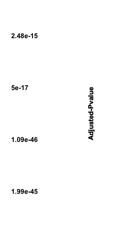
- pvalue subfigure
pl_right_pvalue <- ggplot(data_right, aes(x = Vars, y = estimate, fill = Species)) +
    geom_text(aes(y = 0, x = Vars), label = data_right$adjustP,
              hjust = 0, fontface = "bold", inherit.aes = FALSE, size = 3) +
    geom_text(aes(x = nrow(data_right)/2 + 0.5, y = 0.85), label = "Adjusted-Pvalue",
             srt = 90, fontface = "bold", size = 3) +
    coord_flip() +
    ylim(c(0, 1)) +
    theme(panel.background = element_blank(),
          panel.grid = element_blank(),
          axis.line = element_blank(),
          axis.ticks = element_blank(),
          axis.text = element_blank(),
          axis.title = element_blank())

pl_right_pvalue
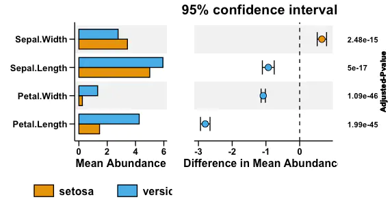
- Combination of all subfigures
pl <- pl_left_bar + pl_right_scatter + pl_right_pvalue +
  plot_layout(widths = c(4, 6, 2))

pl
Conclusion
STAMP is comprise of barplot for mean abundance and error bar plot for hypothesis testing.
Systemic information
devtools::session_info()
## ─ Session info ───────────────────────────────────────────────────────────────
##  setting  value
##  version  R version 4.1.3 (2022-03-10)
##  os       macOS Big Sur/Monterey 10.16
##  system   x86_64, darwin17.0
##  ui       X11
##  language (EN)
##  collate  en_US.UTF-8
##  ctype    en_US.UTF-8
##  tz       Asia/Shanghai
##  date     2023-07-24
##  pandoc   3.1.3 @ /Users/zouhua/opt/anaconda3/bin/ (via rmarkdown)
##
## ─ Packages ───────────────────────────────────────────────────────────────────
##  package     * version date (UTC) lib source
##  backports     1.4.1   2021-12-13 [2] CRAN (R 4.1.0)
##  blogdown      1.18    2023-06-19 [2] CRAN (R 4.1.3)
##  bookdown      0.34    2023-05-09 [2] CRAN (R 4.1.2)
##  broom       * 1.0.5   2023-06-09 [2] CRAN (R 4.1.3)
##  bslib         0.5.0   2023-06-09 [2] CRAN (R 4.1.3)
##  cachem        1.0.8   2023-05-01 [2] CRAN (R 4.1.2)
##  callr         3.7.3   2022-11-02 [2] CRAN (R 4.1.2)
##  cli           3.6.1   2023-03-23 [2] CRAN (R 4.1.2)
##  colorspace    2.1-0   2023-01-23 [2] CRAN (R 4.1.2)
##  crayon        1.5.2   2022-09-29 [2] CRAN (R 4.1.2)
##  devtools      2.4.5   2022-10-11 [2] CRAN (R 4.1.2)
##  digest        0.6.33  2023-07-07 [1] CRAN (R 4.1.3)
##  dplyr       * 1.1.2   2023-04-20 [2] CRAN (R 4.1.2)
##  ellipsis      0.3.2   2021-04-29 [2] CRAN (R 4.1.0)
##  evaluate      0.21    2023-05-05 [2] CRAN (R 4.1.2)
##  fansi         1.0.4   2023-01-22 [2] CRAN (R 4.1.2)
##  farver        2.1.1   2022-07-06 [2] CRAN (R 4.1.2)
##  fastmap       1.1.1   2023-02-24 [2] CRAN (R 4.1.2)
##  forcats     * 1.0.0   2023-01-29 [2] CRAN (R 4.1.2)
##  fs            1.6.2   2023-04-25 [2] CRAN (R 4.1.2)
##  generics      0.1.3   2022-07-05 [2] CRAN (R 4.1.2)
##  ggplot2     * 3.4.2   2023-04-03 [2] CRAN (R 4.1.2)
##  glue          1.6.2   2022-02-24 [2] CRAN (R 4.1.2)
##  gtable        0.3.3   2023-03-21 [2] CRAN (R 4.1.2)
##  highr         0.10    2022-12-22 [2] CRAN (R 4.1.2)
##  hms           1.1.3   2023-03-21 [2] CRAN (R 4.1.2)
##  htmltools     0.5.5   2023-03-23 [2] CRAN (R 4.1.2)
##  htmlwidgets   1.6.2   2023-03-17 [2] CRAN (R 4.1.2)
##  httpuv        1.6.11  2023-05-11 [2] CRAN (R 4.1.3)
##  jquerylib     0.1.4   2021-04-26 [2] CRAN (R 4.1.0)
##  jsonlite      1.8.7   2023-06-29 [2] CRAN (R 4.1.3)
##  knitr         1.43    2023-05-25 [2] CRAN (R 4.1.3)
##  labeling      0.4.2   2020-10-20 [2] CRAN (R 4.1.0)
##  later         1.3.1   2023-05-02 [2] CRAN (R 4.1.2)
##  lifecycle     1.0.3   2022-10-07 [2] CRAN (R 4.1.2)
##  lubridate   * 1.9.2   2023-02-10 [2] CRAN (R 4.1.2)
##  magrittr      2.0.3   2022-03-30 [2] CRAN (R 4.1.2)
##  memoise       2.0.1   2021-11-26 [2] CRAN (R 4.1.0)
##  mime          0.12    2021-09-28 [2] CRAN (R 4.1.0)
##  miniUI        0.1.1.1 2018-05-18 [2] CRAN (R 4.1.0)
##  munsell       0.5.0   2018-06-12 [2] CRAN (R 4.1.0)
##  patchwork   * 1.1.2   2022-08-19 [2] CRAN (R 4.1.2)
##  pillar        1.9.0   2023-03-22 [2] CRAN (R 4.1.2)
##  pkgbuild      1.4.2   2023-06-26 [2] CRAN (R 4.1.3)
##  pkgconfig     2.0.3   2019-09-22 [2] CRAN (R 4.1.0)
##  pkgload       1.3.2.1 2023-07-08 [2] CRAN (R 4.1.3)
##  prettyunits   1.1.1   2020-01-24 [2] CRAN (R 4.1.0)
##  processx      3.8.2   2023-06-30 [2] CRAN (R 4.1.3)
##  profvis       0.3.8   2023-05-02 [2] CRAN (R 4.1.2)
##  promises      1.2.0.1 2021-02-11 [2] CRAN (R 4.1.0)
##  ps            1.7.5   2023-04-18 [2] CRAN (R 4.1.2)
##  purrr       * 1.0.1   2023-01-10 [2] CRAN (R 4.1.2)
##  R6            2.5.1   2021-08-19 [2] CRAN (R 4.1.0)
##  Rcpp          1.0.11  2023-07-06 [1] CRAN (R 4.1.3)
##  readr       * 2.1.4   2023-02-10 [2] CRAN (R 4.1.2)
##  remotes       2.4.2   2021-11-30 [2] CRAN (R 4.1.0)
##  rlang         1.1.1   2023-04-28 [2] CRAN (R 4.1.2)
##  rmarkdown     2.23    2023-07-01 [2] CRAN (R 4.1.3)
##  rstudioapi    0.15.0  2023-07-07 [2] CRAN (R 4.1.3)
##  sass          0.4.6   2023-05-03 [2] CRAN (R 4.1.2)
##  scales        1.2.1   2022-08-20 [2] CRAN (R 4.1.2)
##  sessioninfo   1.2.2   2021-12-06 [2] CRAN (R 4.1.0)
##  shiny         1.7.4.1 2023-07-06 [2] CRAN (R 4.1.3)
##  stringi       1.7.12  2023-01-11 [2] CRAN (R 4.1.2)
##  stringr     * 1.5.0   2022-12-02 [2] CRAN (R 4.1.2)
##  tibble      * 3.2.1   2023-03-20 [2] CRAN (R 4.1.2)
##  tidyr       * 1.3.0   2023-01-24 [2] CRAN (R 4.1.2)
##  tidyselect    1.2.0   2022-10-10 [2] CRAN (R 4.1.2)
##  tidyverse   * 2.0.0   2023-02-22 [1] CRAN (R 4.1.2)
##  timechange    0.2.0   2023-01-11 [2] CRAN (R 4.1.2)
##  tzdb          0.4.0   2023-05-12 [2] CRAN (R 4.1.3)
##  urlchecker    1.0.1   2021-11-30 [2] CRAN (R 4.1.0)
##  usethis       2.2.2   2023-07-06 [2] CRAN (R 4.1.3)
##  utf8          1.2.3   2023-01-31 [2] CRAN (R 4.1.2)
##  vctrs         0.6.3   2023-06-14 [1] CRAN (R 4.1.3)
##  withr         2.5.0   2022-03-03 [2] CRAN (R 4.1.2)
##  xfun          0.39    2023-04-20 [2] CRAN (R 4.1.2)
##  xtable        1.8-4   2019-04-21 [2] CRAN (R 4.1.0)
##  yaml          2.3.7   2023-01-23 [2] CRAN (R 4.1.2)
##
##  [1] /Users/zouhua/Library/R/x86_64/4.1/library
##  [2] /Library/Frameworks/R.framework/Versions/4.1/Resources/library
##
## ──────────────────────────────────────────────────────────────────────────────
Reference
Hua Zou
Senior Bioinformatic Analyst
My research interests include host-microbiota intersection, machine learning and multi-omics data integration.