R visualization: donut chart by ggplot2

donut chart shows the number or proportion per group

Last updated on Jul 14, 2023 9 min read Visualization, ggplot2

Introduction

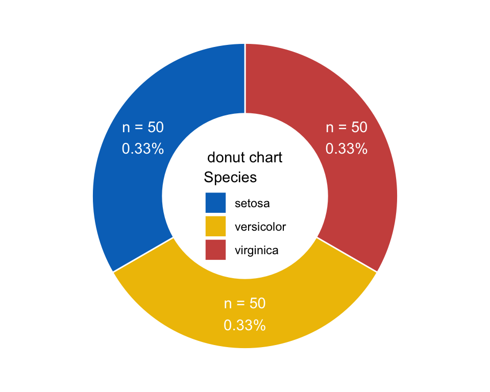
Compared to pie chart, donut chart has one more hole inside. In addition, multiple circles plot shows different traits of dataset.

Loading required packages

knitr::opts_chunk$set(message = FALSE, warning = FALSE)

library(ggplot2) 
library(dplyr)
library(tidyverse)

# group & color
group_names <- c("setosa", "versicolor", "virginica")
group_colors <- c("#0073C2FF", "#EFC000FF", "#CD534CFF")

Data preparation

Loading iris dataset
Summarizing the total number per species
Calculating proportion per species
Computing position of text label

data("iris")

plotdata <- iris |>
  dplyr::group_by(Species) |>
  dplyr::summarise(count = length(Species)) |>
  dplyr::mutate(prop = round(count / sum(count), 2)) |>
  dplyr::arrange(desc(Species)) |>
  dplyr::mutate(lab.ypos = cumsum(prop) - 0.5 * prop) |>
  dplyr::mutate(num_prop = paste0("n = ", count, "\n", 
                           paste0(prop, "%"))) |>
  dplyr::mutate(Species = factor(Species, levels = group_names))

head(plotdata)

## # A tibble: 3 × 5
##   Species    count  prop lab.ypos num_prop       
##   <fct>      <int> <dbl>    <dbl> <chr>          
## 1 virginica     50  0.33    0.165 "n = 50\n0.33%"
## 2 versicolor    50  0.33    0.495 "n = 50\n0.33%"
## 3 setosa        50  0.33    0.825 "n = 50\n0.33%"

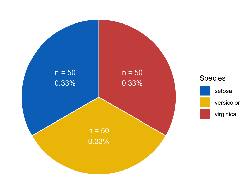
Pie

pie <- ggplot(plotdata, aes(x = "", y = prop, fill = Species)) +
  geom_bar(stat = "identity", color = "white", width = 1) +
  coord_polar(theta = "y", start = 0) +
  geom_text(aes(y = lab.ypos, label = num_prop), color = "white") +
  scale_fill_manual(breaks = group_names,
                    values = group_colors) +
  theme_void()

pie

Donut

donut <- ggplot(plotdata, aes(x = 2, y = prop, fill = Species)) +
  geom_bar(stat = "identity", color = "white") +
  coord_polar(theta = "y", start = 0) +
  geom_text(aes(y = lab.ypos, label = num_prop), color = "white") +
  scale_fill_manual(breaks = group_names,
                    values = group_colors) +
  annotate("text", x = 1, y = 0, label = "donut chart") +
  theme_void() +
  xlim(0.5, 2.5) +
  theme(legend.position = c(.5, .45))

donut

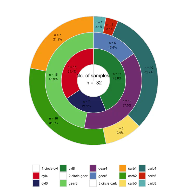
Mulitple circles chart

One circle represents one traits of dataset, should we using multiple circles to characterize the different traits?

Traits of mtcars: cyl, gear and carb

Data preparation

data_select <- mtcars |>
  dplyr::select(cyl, gear, carb) |>
  mutate_if(is.numeric, as.character) |>
  mutate_if(is.character, as.factor) |>
  mutate(cyl = paste0("cyl", cyl),
         gear = paste0("gear", gear),
         carb = paste0("carb", carb))

str(data_select)

## 'data.frame':	32 obs. of  3 variables:
##  $ cyl : chr  "cyl6" "cyl6" "cyl4" "cyl6" ...
##  $ gear: chr  "gear4" "gear4" "gear4" "gear3" ...
##  $ carb: chr  "carb4" "carb4" "carb1" "carb1" ...

Calculating the Proportion per group

plotdata2 <- data_select |>
  dplyr::group_by(cyl, gear, carb) |>
  dplyr::summarise(count = length(cyl)) 

head(plotdata2)

## # A tibble: 6 × 4
## # Groups:   cyl, gear [5]
##   cyl   gear  carb  count
##   <chr> <chr> <chr> <int>
## 1 cyl4  gear3 carb1     1
## 2 cyl4  gear4 carb1     4
## 3 cyl4  gear4 carb2     4
## 4 cyl4  gear5 carb2     2
## 5 cyl6  gear3 carb1     2
## 6 cyl6  gear4 carb4     4

Function for drawing chart
- single or multiple traits for plotting
- values and position of label
- plotting

get_circle <- function(
    inputdata,
    variables = c("cyl", "gear", "carb"),
    label_size = 2.5,
    annotate_size = 4,
    col_number = 5,
    theme_legend_size = 8,
    theme_strip_size = 8,
    axis_size = 10,
    cyl_names = c("cyl4", "cyl6","cyl8"),
    cyl_cols = c("#D51F26", "#272E6A", "#208A42"),
    gear_names = c("gear3", "gear4", "gear5"),
    gear_cols = c("#7DD06F", "#844081", "#688EC1"),
    carb_names = c("carb1", "carb2", "carb3", "carb4", "carb6", "carb8"),
    carb_cols = c("#faa818", "#41a30d", "#fbdf72", "#367d7d", "#d33502", "#6ebcbc")) {
  
  dat_list <- list()
  for (i in 1:length(variables)) {
    temp_var <- rlang::sym(variables[i])
    temp_dat <- inputdata %>%
      dplyr::select(!!temp_var, count) %>%
      dplyr::group_by(!!temp_var) %>%
      dplyr::summarise(count = sum(count), .groups = "drop")      
    dat_list[[i]] <- temp_dat
  }
  
  names(dat_list) <- variables
  
  get_plotdata <- function(dat) {
    
    dat_cln_list <- list()
    names_new_list <- list()
    colors_new_list <- list()
    
    for (i in 1:length(dat)) {
      if (names(dat)[i] == "cyl") {
        cyl_cln <- dat[[i]] %>%
          dplyr::select(cyl, count) %>%
          dplyr::group_by(cyl) %>%
          dplyr::summarise(count = sum(count)) %>%
          dplyr::mutate(prop = round(count / sum(count), 3) * 100) %>%
          dplyr::ungroup() %>%
          dplyr::arrange(desc(cyl)) %>%
          dplyr::mutate(lab.ypos = cumsum(prop) - 0.5*prop) %>%
          dplyr::mutate(num_prop = paste0("n = ", count, "\n", 
                                          paste0(prop, "%")))
        cyl_cln$level <- i 
        cyl_cln$type <- "cyl"
        match_order_index1 <- sort(pmatch(unique(cyl_cln$cyl), cyl_names), decreasing = F)
        cyl_names_new <- cyl_names[match_order_index1]
        cyl_cols_new <- cyl_cols[match_order_index1]     
        cyl_cln$fill <- factor(cyl_cln$cyl, levels = cyl_names_new, labels = cyl_cols_new)
        
        dat_cln_list[[i]] <- cyl_cln
        names_new_list[[i]] <- cyl_names_new
        colors_new_list[[i]] <- cyl_cols_new
        
      } else if (names(dat)[i] == "gear") {
        gear_cln <- dat[[i]] %>%
          dplyr::select(gear, count) %>%
          dplyr::group_by(gear) %>%
          dplyr::summarise(count = sum(count)) %>%
          dplyr::mutate(prop = round(count / sum(count), 3) * 100) %>%
          dplyr::ungroup() %>%
          dplyr::arrange(desc(gear)) %>%
          dplyr::mutate(lab.ypos = cumsum(prop) - 0.5*prop) %>%
          dplyr::mutate(num_prop = paste0("n = ", count, "\n", 
                                          paste0(prop, "%")))
        gear_cln$level <- i
        gear_cln$type <- "gear"
        match_order_index2 <- sort(pmatch(unique(gear_cln$gear), gear_names), decreasing = F)    
        gear_names_new <- gear_names[match_order_index2]
        gear_cols_new <- gear_cols[match_order_index2]     
        gear_cln$fill <- factor(gear_cln$gear, levels = gear_names_new, labels = gear_cols_new)
        
        dat_cln_list[[i]] <- gear_cln
        names_new_list[[i]] <- gear_names_new
        colors_new_list[[i]] <- gear_cols_new
        
      } else if (names(dat)[i] == "carb") {
        carb_cln <- dat[[i]] %>%
          dplyr::select(carb, count) %>%
          dplyr::group_by(carb) %>%
          dplyr::summarise(count = sum(count)) %>%
          dplyr::mutate(prop = round(count / sum(count), 3) * 100) %>%
          dplyr::ungroup() %>%
          dplyr::arrange(desc(carb)) %>%
          dplyr::mutate(lab.ypos = cumsum(prop) - 0.5*prop) %>%
          dplyr::mutate(num_prop = paste0("n = ", count, "\n", 
                                          paste0(prop, "%"))) 
        carb_cln$level <- i
        carb_cln$type <- "carb"
        match_order_index3 <- sort(pmatch(unique(carb_cln$carb), carb_names), decreasing = F)    
        carb_names_new <- carb_names[match_order_index3]
        carb_cols_new <- carb_cols[match_order_index3]     
        carb_cln$fill <- factor(carb_cln$carb, levels = carb_names_new, labels = carb_cols_new)
        
        dat_cln_list[[i]] <- carb_cln
        names_new_list[[i]] <- carb_names_new
        colors_new_list[[i]] <- carb_cols_new
        
      }
    }
    
    names(dat_cln_list) <- names(dat)
    names(names_new_list) <- names(dat)
    names(colors_new_list) <- names(dat)
    
    temp_name <- c()
    temp_value <- c()
    temp_level <- c()
    temp_type <- c()
    temp_num_prop <- c()
    for (j in 1:length(dat_cln_list)) {
      temp_name <- c(temp_name, dat_cln_list[[j]][, 1, T])
      temp_value <- c(temp_value, dat_cln_list[[j]][, 2, T])
      temp_level <- c(temp_level, dat_cln_list[[j]][, 6, T])
      temp_type <- c(temp_type, dat_cln_list[[j]][, 7, T])
      temp_num_prop <- c(temp_num_prop, dat_cln_list[[j]][, 5, T])
    }
    
    data_temp <- data.frame(name = temp_name,
                            value = temp_value,
                            level = temp_level,
                            type = temp_type,
                            num_prop = temp_num_prop)
    data_parent <- data.frame(name = "Parent", value = 0, level = 0, type = NA, num_prop = NA)
    dat_res <- rbind(data_parent, data_temp)
    res <- list(plotdata = dat_res,
                names_new = names_new_list,
                colors_new = colors_new_list)
    
    return(res)
  }
  
  # discrete variables
  res_list <- get_plotdata(dat = dat_list)
  plotdata <- res_list$plotdata
  
  name_levels <- c()
  name_colors <- c()
  for (k in 1:length(res_list$names_new)) {
    temp_name <- c(paste(k, "circle", names(res_list$names_new)[k]), res_list$names_new[[k]])
    temp_color <- c("white", res_list$colors_new[[k]])
    
    name_levels <- c(name_levels, temp_name)
    name_colors <- c(name_colors, temp_color)
  }
  
  names(name_colors) <- name_levels
  
  plotdata$name <- factor(plotdata$name, levels = name_levels)
  total_num <- plotdata %>%
    dplyr::pull(value) %>%
    sum() / length(variables)
  
  pl <- ggplot(plotdata, aes(x = level, y = value, fill = name)) + 
    geom_col(width = 1, color = "gray90", size = 0.5, position = position_stack()) +
    geom_text(aes(label = num_prop), size = label_size, position = position_stack(vjust = 0.5)) +
    coord_polar(theta = "y", start = 0) +
    scale_x_discrete(breaks = NULL) +
    scale_y_continuous(breaks = NULL) +
    labs(x = NULL, y = NULL) +  
    scale_fill_manual(values = name_colors, drop = FALSE) +
    guides(fill = guide_legend(title = NULL, ncol = col_number)) +
    annotate("text", x = -0.4, y = 0, 
             label = paste("No. of samples", "\n n = ", total_num), 
             size = annotate_size) +
    theme_void() +
    theme(axis.title = element_text(face = "bold", size = axis_size),
          axis.text = element_text(size = axis_size - 1),
          text = element_text(size = axis_size - 2),
          legend.position = "bottom",
          legend.text = element_text(size = theme_legend_size, color = "black"),
          strip.text.x = element_text(size = theme_strip_size, color = "black", face = "bold"))
  
  return(pl)
}

multiple circles

pl_circle <- get_circle(
    inputdata = plotdata2,
    variables = c("cyl", "gear", "carb"),
    label_size = 2.5,
    annotate_size = 4,
    col_number = 5,
    theme_legend_size = 8,
    theme_strip_size = 8,
    axis_size = 10)

pl_circle

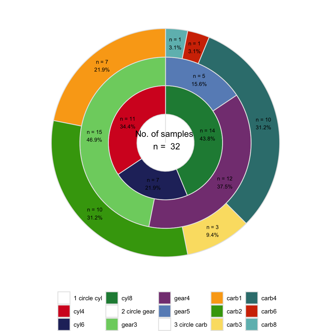
Conclusion

Pie and donut only are fit for proportion of single variable, while multiple circles are suitable for ratio of multiple traits in dataset.

Systemic information

devtools::session_info()

## ─ Session info ───────────────────────────────────────────────────────────────
##  setting  value
##  version  R version 4.1.3 (2022-03-10)
##  os       macOS Big Sur/Monterey 10.16
##  system   x86_64, darwin17.0
##  ui       X11
##  language (EN)
##  collate  en_US.UTF-8
##  ctype    en_US.UTF-8
##  tz       Asia/Shanghai
##  date     2023-07-24
##  pandoc   3.1.3 @ /Users/zouhua/opt/anaconda3/bin/ (via rmarkdown)
## 
## ─ Packages ───────────────────────────────────────────────────────────────────
##  package     * version date (UTC) lib source
##  blogdown      1.18    2023-06-19 [2] CRAN (R 4.1.3)
##  bookdown      0.34    2023-05-09 [2] CRAN (R 4.1.2)
##  bslib         0.5.0   2023-06-09 [2] CRAN (R 4.1.3)
##  cachem        1.0.8   2023-05-01 [2] CRAN (R 4.1.2)
##  callr         3.7.3   2022-11-02 [2] CRAN (R 4.1.2)
##  cli           3.6.1   2023-03-23 [2] CRAN (R 4.1.2)
##  colorspace    2.1-0   2023-01-23 [2] CRAN (R 4.1.2)
##  crayon        1.5.2   2022-09-29 [2] CRAN (R 4.1.2)
##  devtools      2.4.5   2022-10-11 [2] CRAN (R 4.1.2)
##  digest        0.6.33  2023-07-07 [1] CRAN (R 4.1.3)
##  dplyr       * 1.1.2   2023-04-20 [2] CRAN (R 4.1.2)
##  ellipsis      0.3.2   2021-04-29 [2] CRAN (R 4.1.0)
##  evaluate      0.21    2023-05-05 [2] CRAN (R 4.1.2)
##  fansi         1.0.4   2023-01-22 [2] CRAN (R 4.1.2)
##  farver        2.1.1   2022-07-06 [2] CRAN (R 4.1.2)
##  fastmap       1.1.1   2023-02-24 [2] CRAN (R 4.1.2)
##  forcats     * 1.0.0   2023-01-29 [2] CRAN (R 4.1.2)
##  fs            1.6.2   2023-04-25 [2] CRAN (R 4.1.2)
##  generics      0.1.3   2022-07-05 [2] CRAN (R 4.1.2)
##  ggplot2     * 3.4.2   2023-04-03 [2] CRAN (R 4.1.2)
##  glue          1.6.2   2022-02-24 [2] CRAN (R 4.1.2)
##  gtable        0.3.3   2023-03-21 [2] CRAN (R 4.1.2)
##  highr         0.10    2022-12-22 [2] CRAN (R 4.1.2)
##  hms           1.1.3   2023-03-21 [2] CRAN (R 4.1.2)
##  htmltools     0.5.5   2023-03-23 [2] CRAN (R 4.1.2)
##  htmlwidgets   1.6.2   2023-03-17 [2] CRAN (R 4.1.2)
##  httpuv        1.6.11  2023-05-11 [2] CRAN (R 4.1.3)
##  jquerylib     0.1.4   2021-04-26 [2] CRAN (R 4.1.0)
##  jsonlite      1.8.7   2023-06-29 [2] CRAN (R 4.1.3)
##  knitr         1.43    2023-05-25 [2] CRAN (R 4.1.3)
##  labeling      0.4.2   2020-10-20 [2] CRAN (R 4.1.0)
##  later         1.3.1   2023-05-02 [2] CRAN (R 4.1.2)
##  lifecycle     1.0.3   2022-10-07 [2] CRAN (R 4.1.2)
##  lubridate   * 1.9.2   2023-02-10 [2] CRAN (R 4.1.2)
##  magrittr      2.0.3   2022-03-30 [2] CRAN (R 4.1.2)
##  memoise       2.0.1   2021-11-26 [2] CRAN (R 4.1.0)
##  mime          0.12    2021-09-28 [2] CRAN (R 4.1.0)
##  miniUI        0.1.1.1 2018-05-18 [2] CRAN (R 4.1.0)
##  munsell       0.5.0   2018-06-12 [2] CRAN (R 4.1.0)
##  pillar        1.9.0   2023-03-22 [2] CRAN (R 4.1.2)
##  pkgbuild      1.4.2   2023-06-26 [2] CRAN (R 4.1.3)
##  pkgconfig     2.0.3   2019-09-22 [2] CRAN (R 4.1.0)
##  pkgload       1.3.2.1 2023-07-08 [2] CRAN (R 4.1.3)
##  prettyunits   1.1.1   2020-01-24 [2] CRAN (R 4.1.0)
##  processx      3.8.2   2023-06-30 [2] CRAN (R 4.1.3)
##  profvis       0.3.8   2023-05-02 [2] CRAN (R 4.1.2)
##  promises      1.2.0.1 2021-02-11 [2] CRAN (R 4.1.0)
##  ps            1.7.5   2023-04-18 [2] CRAN (R 4.1.2)
##  purrr       * 1.0.1   2023-01-10 [2] CRAN (R 4.1.2)
##  R6            2.5.1   2021-08-19 [2] CRAN (R 4.1.0)
##  Rcpp          1.0.11  2023-07-06 [1] CRAN (R 4.1.3)
##  readr       * 2.1.4   2023-02-10 [2] CRAN (R 4.1.2)
##  remotes       2.4.2   2021-11-30 [2] CRAN (R 4.1.0)
##  rlang         1.1.1   2023-04-28 [2] CRAN (R 4.1.2)
##  rmarkdown     2.23    2023-07-01 [2] CRAN (R 4.1.3)
##  rstudioapi    0.15.0  2023-07-07 [2] CRAN (R 4.1.3)
##  sass          0.4.6   2023-05-03 [2] CRAN (R 4.1.2)
##  scales        1.2.1   2022-08-20 [2] CRAN (R 4.1.2)
##  sessioninfo   1.2.2   2021-12-06 [2] CRAN (R 4.1.0)
##  shiny         1.7.4.1 2023-07-06 [2] CRAN (R 4.1.3)
##  stringi       1.7.12  2023-01-11 [2] CRAN (R 4.1.2)
##  stringr     * 1.5.0   2022-12-02 [2] CRAN (R 4.1.2)
##  tibble      * 3.2.1   2023-03-20 [2] CRAN (R 4.1.2)
##  tidyr       * 1.3.0   2023-01-24 [2] CRAN (R 4.1.2)
##  tidyselect    1.2.0   2022-10-10 [2] CRAN (R 4.1.2)
##  tidyverse   * 2.0.0   2023-02-22 [1] CRAN (R 4.1.2)
##  timechange    0.2.0   2023-01-11 [2] CRAN (R 4.1.2)
##  tzdb          0.4.0   2023-05-12 [2] CRAN (R 4.1.3)
##  urlchecker    1.0.1   2021-11-30 [2] CRAN (R 4.1.0)
##  usethis       2.2.2   2023-07-06 [2] CRAN (R 4.1.3)
##  utf8          1.2.3   2023-01-31 [2] CRAN (R 4.1.2)
##  vctrs         0.6.3   2023-06-14 [1] CRAN (R 4.1.3)
##  withr         2.5.0   2022-03-03 [2] CRAN (R 4.1.2)
##  xfun          0.39    2023-04-20 [2] CRAN (R 4.1.2)
##  xtable        1.8-4   2019-04-21 [2] CRAN (R 4.1.0)
##  yaml          2.3.7   2023-01-23 [2] CRAN (R 4.1.2)
## 
##  [1] /Users/zouhua/Library/R/x86_64/4.1/library
##  [2] /Library/Frameworks/R.framework/Versions/4.1/Resources/library
## 
## ──────────────────────────────────────────────────────────────────────────────

Reference

HOW TO CREATE A PIE CHART IN R USING GGPLOT2

Visualization