Multiple approaches for identification of microbial biomarkers
Differential analysis in metagenomics

Introduction
Identifying species that differ between groups is a common data analysis in the field of microbiology. We used three different types of difference analysis to discover significantly different microbial species (Derosa et al. 2022), they are:
Linear Discriminant Analysis of Effect Size (LefSe).
Microbiome Multivariable Association with Linear Models (Maaslin2).
Analysis of Composition of Microbiomes with Bias Correction (ANCOM-BC).
LefSe is a method based on supervised linear discriminant screening of discrepant species; Maaslin2 is a method based on a linear regression algorithm for identifying discrepant species; and ANCOM-BC is a method for correcting for absolute abundance bias between samples and zero-value inflation, among others, before discovering discrepant species.
We will use the differential species identified by LefSe as a benchmark, merge the differential results of the other two methods, and finally present the results in a bar chart.
MicrobiomeAnalysis installation
MicrobiomeAnalysis will provide the following functions for downstream data analysis.
if (!requireNamespace(c("remotes", "devtools"), quietly=TRUE)) {
  install.packages(c("devtools", "remotes"))
}
remotes::install_github("HuaZou/MicrobiomeAnalysis")
Loading required packages
R packages in this tutorial.
knitr::opts_chunk$set(message = FALSE, warning = FALSE)
library(tidyverse)
library(MicrobiomeAnalysis)
library(Maaslin2)
library(ANCOMBC)
library(phyloseq)
library(ggpubr)

# rm(list = ls())
options(stringsAsFactors = F)
options(future.globals.maxSize = 1000 * 1024^2)

# group & color
sex_grp <- c("Male", "Female")
sex_col <- c("#F28880", "#60C4D3")

lf_grp <- c("None", "Mild", "Moderate", "Severe")
lf_col <- c("#803C08", "#F1A340", "#2C0a4B", "#998EC3")
Data preparation
Data were obtained from the gut microbiology data of Zeybel_2022 and can be accessed in MicrobiomeAnalysis.
phy <- MicrobiomeAnalysis::Zeybel_2022_gut
phy
## phyloseq-class experiment-level object
## otu_table()   OTU Table:         [ 547 taxa and 42 samples ]
## sample_data() Sample Data:       [ 42 samples by 46 sample variables ]
## tax_table()   Taxonomy Table:    [ 547 taxa by 7 taxonomic ranks ]
The data object phy consists of three components: an otu table in species level, a metadata table, and a table with multiple taxonomic levels.
colnames(phy@sam_data)[1:4]
## [1] "Gender"             "Age"                "LiverFatClass"
## [4] "AlcoholConsumption"
Using LiverFatClass as the comparison group and Gender, Age as the confounding factors.
Because there is no absolute abundance table, the relative abundance table is converted to absolute abundance table for the time being (note: accurate absolute abundance table is required, amplicons can be used with counts, Metaphlan series can be used with counts such as FPKM).
phy_count <- phyloseq::transform_sample_counts(
  phy, function(x){round(x*10^7, 0)})

# head(otu_table(phy_count), 4)
Linear Discriminant Analysis of Effect Size (LefSe)
Provide encapsulated function for calculation and plotting.
get_lefse: Obtaining the LefSe result;
get_lefse_pl: Plotting the result;
get_boxplot: the boxplot between groups.
get_lefse <- function(
  ps,
  taxa_level = c(NULL, "Phylum", "Class", "Order",
                 "Family", "Genus", "Species"),
  filterCol = NULL,
  filterVars = NULL,
  group = c("LiverFatClass", "Gender"),
  group_names = c("None", "Mild", "Moderate", "Severe",
                  "Male", "Female"),
  prev_cutoff = 0.1,
  mean_threshold = 0.0001,
  one_threshold = 0.001,
  LDA_cutoff = 2) {

  # ps = phy
  # taxa_level = NULL
  # filterCol = NULL
  # filterVars = NULL
  # group = "LiverFatClass"
  # group_names = c("None", "Mild")
  # prev_cutoff = 0.1
  # mean_threshold = 0.0001
  # one_threshold = 0.001
  # LDA_cutoff = 0


  if (!is.null(taxa_level)) {
    ps_taxa <- MicrobiomeAnalysis::aggregate_taxa(
      x = ps, level = taxa_level)
  } else {
    ps_taxa <- ps
  }

  metadata <- ps_taxa@sam_data %>%
    data.frame()

  if (is.null(filterCol)) {
    dat_cln <- metadata
  } else {
    colnames(metadata)[which(colnames(metadata) == filterCol)] <- "FiltCol"
    dat_cln <- metadata %>%
      dplyr::filter(FiltCol %in% filterVars)
    colnames(metadata)[which(colnames(metadata) == "FiltCol")] <- filterCol
  }

  # group for test
  dat_cln2 <- dat_cln
  colnames(dat_cln2)[which(colnames(dat_cln2) == group)] <- "Group_new"
  if (group_names[1] == "all") {
    dat_cln3 <- dat_cln2
  } else {
    dat_cln3 <- dat_cln2 %>%
      dplyr::filter(Group_new %in% group_names)
  }

  dat_cln3$Group_new <- factor(dat_cln3$Group_new, levels = group_names)
  colnames(dat_cln3)[which(colnames(dat_cln3) == "Group_new")] <- group

  ps_temp <- ps_taxa
  phyloseq::sample_data(ps_temp) <- phyloseq::sample_data(dat_cln3)

  # trim & filter
  ps_trim <- MicrobiomeAnalysis::trim_prevalence(
    object = ps_temp,
    cutoff = prev_cutoff,
    trim = "feature")
  ps_filter <- MicrobiomeAnalysis::filter_abundance(
    object = ps_trim,
    cutoff_mean = mean_threshold,
    cutoff_one = one_threshold)

  # run lefse
  set.seed(123)
  res_lefse <- MicrobiomeAnalysis::run_lefse(
                    ps = ps_filter,
                    group = group,
                    taxa_rank = "none",
                    norm = "CPM",
                    lda_cutoff = LDA_cutoff)

  res_lda <- res_lefse@marker_table %>%
    data.frame() %>%
    dplyr::inner_join(ps_filter@tax_table %>%
                        data.frame() %>%
                        tibble::rownames_to_column("feature"),
                      by = "feature")
  # Number of Group
  input_metadata <- ps_filter@sam_data %>%
    data.frame()
  colnames(input_metadata)[which(colnames(input_metadata) == group)] <- "Compvar"
  dat_status <- table(input_metadata$Compvar)
  dat_status_number <- as.numeric(dat_status)
  dat_status_name <- names(dat_status)
  res_lda$Block <- paste(paste(dat_status_number[1], dat_status_name[1], sep = "_"),
                       "vs",
                       paste(dat_status_number[2], dat_status_name[2], sep = "_"))
  res_DA <- res_lda %>%
    dplyr::rename(TaxaID = feature,
                  Enrichment = enrich_group,
                  LDA_Score = ef_lda) %>%
    dplyr::mutate(LDA_Score = ifelse(Enrichment == group_names[1],
                                     -LDA_Score, LDA_Score)) %>%
    dplyr::select(TaxaID, Block, everything())


  # final results list
  res <- list(ps = ps_filter,
              test_res = res_DA)

  return(res)
}

get_lefse_pl <- function(
  dat,
  index,
  cutoff = 2,
  group_color) {

  # dat = res_DA
  # index = "LDA_Score"
  # cutoff = 2
  # group_color = lf_col[c(1, 4)]


  plot_lefse <- function(
    da_res,
    group_names = NULL,
    x_index,
    x_index_cutoff = 2,
    group_color = c("green", "red"),
    line_size = 0.6,
    theme_text_size = 10,
    theme_title_size = 12,
    theme_legend_size = 12) {

    # group
    da_res_group_names <- gsub("\\d+_", "", unlist(strsplit(da_res$Block[1], " vs ")))
    if (is.null(group_names)) {
      group_names <- da_res_group_names
    } else {
      if (!all(group_names == da_res_group_names)) {
        message("group names are in wrong order, and reoder them")
        group_names <- da_res_group_names
      }else{
        group_names <- group_names
      }
    }

    if (!x_index %in% colnames(da_res)) {
      stop("No x_index matched the DA results' column, please check out your inputdata")
    }
    colnames(da_res)[which(colnames(da_res) == x_index)] <- "Xindex"
    # significant results

    # enrichment by new LDA cutoff
    da_res[which(da_res$Xindex > x_index_cutoff), "EnrichedDir"] <- group_names[2]
    da_res[which(da_res$Xindex < -x_index_cutoff), "EnrichedDir"] <- group_names[1]
    da_res[which(abs(da_res$Xindex) <= x_index_cutoff), "EnrichedDir"] <- "Nonsignif"
    df_status <- table(da_res$EnrichedDir) %>%
      data.frame() %>%
      stats::setNames(c("Group", "Number"))
    grp1_number <- with(df_status, df_status[Group %in% group_names[1], "Number"])
    grp2_number <- with(df_status, df_status[Group %in% group_names[2], "Number"])
    nsf_number <- with(df_status, df_status[Group %in% "Nonsignif", "Number"])
    legend_label <- c(paste0(group_names[1], " (", grp1_number, ")"),
                      paste0("Nonsignif", " (", nsf_number, ")"),
                      paste0(group_names[2], " (", grp2_number, ")"))

    da_res_signif <- da_res %>%
      dplyr::arrange(Xindex) %>%
      dplyr::filter(abs(Xindex) >= x_index_cutoff)
    if (nrow(da_res_signif) == 0) {
      message("There is no significant taxa matched the threshold of LDA_Score")
    }

    if (!is.null(group_color)) {
      plot_group_color <- group_color
      names(plot_group_color) <- group_names
    } else{
      plot_group_color <- c("green", "red")
      names(plot_group_color) <- group_names
    }

    dat_range <- range(da_res_signif$Xindex)
    if (dat_range[1] > 0) {
      x_range <- c(0, ceiling(dat_range[2]))
      limits <- c(0, range(da_res_signif$Xindex)[2])
    }
    if (dat_range[2] < 0) {
      dat_start <- round(dat_range[1] - 1)
      x_range <- c(dat_start, round(dat_range[2]))
      limits <- c(range(da_res_signif$Xindex)[1], 0)
    }
    if (all(dat_range[1] < 0, dat_range[2] > 0)) {
      dat_start <- round(dat_range[1] - 1)
      x_range <- c(dat_start, ceiling(dat_range[2]))
      limits <- x_range
    }


    break_scale <- sum(abs(ceiling(range(da_res_signif$Xindex)))) / 6
    if (break_scale > 0.5) {
      break_scale_final <- ceiling(break_scale)
    } else {
      break_scale_final <- round(break_scale, 1)
    }
    breaks <- seq(x_range[1], x_range[2], break_scale_final)

    pl <- ggplot(da_res_signif, aes(x = reorder(TaxaID, Xindex), y = Xindex)) +
      geom_bar(stat = "identity", aes(fill = Enrichment),
               color = "black", width = .6) +
      geom_hline(yintercept = 0, alpha = .8, linetype = 1, size = line_size + 0.1) +
      geom_hline(yintercept = breaks[breaks != 0], alpha = .8, linetype = 2, size = line_size) +
      scale_fill_manual(values = plot_group_color) +
      scale_y_continuous(breaks = breaks, limits = limits) +
      ylab(x_index) +
      xlab("") +
      coord_flip() +
      theme_bw() +
      theme(axis.ticks.length = unit(0.4, "lines"),
            axis.ticks = element_line(color = "black"),
            axis.line = element_line(color = "black"),
            axis.title.x = element_text(size = theme_title_size, color = "black", face = "bold"),
            axis.text.x = element_text(size = theme_text_size, color = "black", face = "bold"),
            axis.text.y = element_text(size = theme_text_size, color = "black", face = "italic"),
            legend.title = element_blank(),
            legend.text = element_text(size = theme_legend_size, face = "bold", color = "black",
                                     margin = margin(r = 20)),
            legend.position = c(.76, .05),
            legend.direction = "horizontal",
            legend.key.width = unit(0.8, "cm"),
            legend.key.height = unit(0.5, "cm")
            )

    return(pl)
  }

  pl <- plot_lefse(
    da_res = dat,
    x_index = index,
    x_index_cutoff = cutoff,
    group_color = group_color,
    theme_legend_size = 8) +
    theme(legend.background = element_rect(fill = rgb(1, 1, 1, alpha = 0.001), color = NA))

  return(pl)
}


# plot boxplot
get_boxplot <- function(
  ps,
  feature,
  group = c("LiverFatClass", "Gender"),
  group_names = c("None", "Mild", "Moderate", "Severe",
                  "Male", "Female"),
  group_color,
  pl_title,
  pos_cutoff = -0.002) {

  # ps = lefse_df$ps
  # feature = "s__Dorea_longicatena"
  # group = "LiverFatClass"
  # group_names = c("None", "Mild")
  # group_color = lf_col[c(1, 2)]
  # pl_title = "Dorea_longicatena"
  # pos_cutoff = -0.002

  # metadata
  dat_phe <- phyloseq::sample_data(ps) %>%
    data.frame()

  # group
  colnames(dat_phe)[which(colnames(dat_phe) == group)] <- "Group_new"
  phen <- dat_phe %>%
    dplyr::filter(Group_new %in% group_names) %>%
    dplyr::select(Group_new) %>%
    tibble::rownames_to_column("TempRowNames")

  # features
  prof <- phyloseq::otu_table(ps) %>%
    data.frame() %>% t() %>% data.frame() %>%
    dplyr::select(all_of(feature)) %>%
    tibble::rownames_to_column("TempRowNames")

  plotdata <- phen %>%
    dplyr::inner_join(prof, by = "TempRowNames") %>%
    dplyr::mutate(Group_new = factor(Group_new, levels = group_names))
  colnames(plotdata)[2:3] <- c("Group", "Index")

  occ_cutoff <- 0
  occ_fun <- function(x) {
    return(round(length(x[x > occ_cutoff])/length(x), 4))
  }

  plotOcc <- plotdata |>
    dplyr::group_by(Group) |>
    dplyr::summarise(occ = occ_fun(Index)) |>
    dplyr::mutate(occ_lab = paste0(round(occ, 3) * 100, "%")) |>
    dplyr::mutate(position = min(plotdata$Index) - min(plotdata$Index) * 0.1,
                  position = ifelse(position == 0, pos_cutoff, position))

  pl <- ggplot(data = plotdata, aes(x = Group, y = Index, color = Group)) +
    stat_boxplot(geom = "errorbar", width = 0.15) +
    geom_boxplot(width = .4, outlier.shape = NA) +
    geom_point(size = 2, shape = 5) +
    labs(x = "", y = "Relative Abundance", title = pl_title) +
    scale_y_continuous(expand = expansion(mult = c(0.1, 0.1))) +
    geom_point(data = plotOcc, aes(x = Group, y = position, size = occ),
               show.legend = FALSE, shape = 1, stroke = 1) +
    geom_text(data = plotOcc, aes(x = Group, y = position, label = occ_lab),
              show.legend = FALSE) +
    scale_size_continuous(range = c(10, 12)) +
    coord_flip() +
    guides(color = "none") +
    theme_classic() +
    theme(plot.title = element_text(size = 13, color = "black", face = "bold", hjust = .5),
          axis.title = element_text(size = 12, color = "black", face = "bold"),
          axis.text = element_text(size = 10, color = "black"),
          text = element_text(size = 9, color = "black"))

  return(pl)
}
- Differential Analysis from LefSe
Using LiverFatClass as the comparison group, two subgroups, None and Mild, were selected for difference analysis.
lefse_df <- get_lefse(
  ps = phy,
  taxa_level = NULL,
  filterCol = NULL,
  filterVars = NULL,
  group = "LiverFatClass",
  group_names = c("None", "Mild"),
  prev_cutoff = 0.1,
  mean_threshold = 0.0001,
  one_threshold = 0.001,
  LDA_cutoff = 2)

head(lefse_df$test_res[, 1:5], 3)
##                      TaxaID             Block Enrichment LDA_Score     pvalue
## 1  s__Prevotella_sp_CAG_520 9_None vs 12_Mild       None -4.263390 0.01128208
## 2 s__Prevotella_sp_CAG_5226 9_None vs 12_Mild       None -4.023555 0.04089029
## 3  s__Prevotella_sp_AM42_24 9_None vs 12_Mild       None -3.921591 0.01972625
Result: A total of 16 significantly different species were identified by the lefse approach
- Visualization
lefse_pl <- get_lefse_pl(
  dat = lefse_df$test_res,
  index = "LDA_Score",
  cutoff = 2,
  group_color = lf_col[c(1, 2)])

lefse_pl
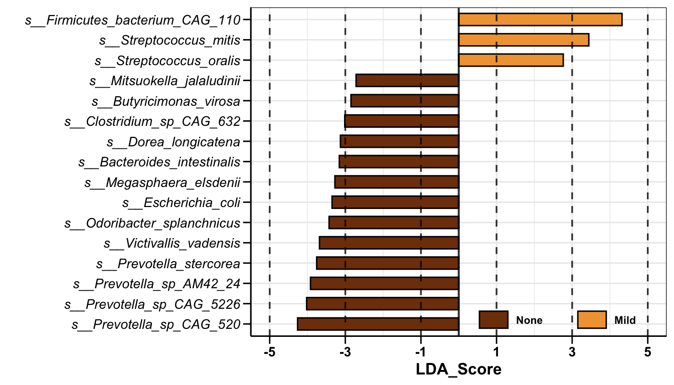
Result: 13 types of differential bacteria were enriched in the None group and 3 types of differential bacteria were enriched in the Mild group.
- Boxplot showing the relative abundance of the specific bacteria
get_boxplot(
  ps = lefse_df$ps,
  feature = "s__Dorea_longicatena",
  group = "LiverFatClass",
  group_names = c("None", "Mild"),
  group_color = lf_col[c(1, 2)],
  pl_title = "Dorea_longicatena",
  pos_cutoff = -0.002)
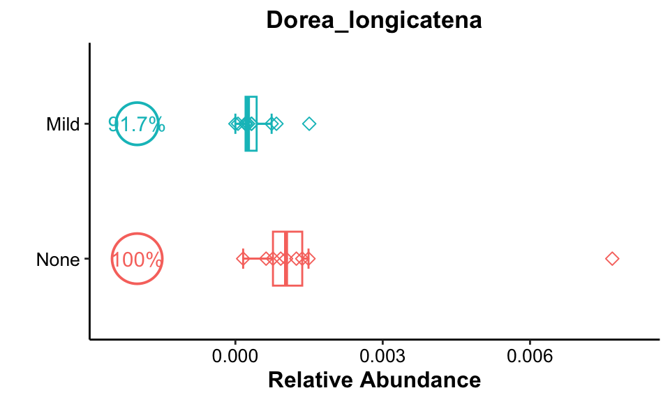
Result: Dorea longicatena had high occurrences (>90%) in both groups, and relative abundance was higher in the None group, but this phenomenon may be due to the rightmost outlier.
Microbiome Multivariable Association with Linear Models (Maaslin2)
Provide encapsulated function for calculation and plotting.
get_Maaslin2: Obtaining the Maaslin2 result;
get_Maaslin2_pl: Plotting the result.
get_Maaslin2 <- function(
  ps,
  taxa_level = c(NULL, "Phylum", "Class", "Order",
                 "Family", "Genus", "Species", "Strain"),
  filterCol = NULL,
  filterVars = NULL,
  group = c("LiverFatClass", "Gender"),
  group_names = c("None", "Mild", "Moderate", "Severe",
                  "Male", "Female"),
  prev_cutoff = 0.1,
  mean_threshold = 0.0001,
  one_threshold = 0.001,
  fix_vars = c("Age", "Gender"),
  outputname) {

  # ps = phy
  # taxa_level = NULL
  # filterCol = NULL
  # filterVars = NULL
  # group = "LiverFatClass"
  # group_names = c("None", "Mild")
  # prev_cutoff = 0.1
  # mean_threshold = 0.0001
  # one_threshold = 0.001
  # fix_vars = c("Age", "Gender")
  # outputname = "LiverFatClass_NM"

  if (!is.null(taxa_level)) {
    ps_taxa <- MicrobiomeAnalysis::aggregate_taxa(
      x = ps, level = taxa_level)
  } else {
    ps_taxa <- ps
  }

  metadata <- ps_taxa@sam_data %>%
    data.frame()

  if (is.null(filterCol)) {
    dat_cln <- metadata
  } else {
    colnames(metadata)[which(colnames(metadata) == filterCol)] <- "FiltCol"
    dat_cln <- metadata %>%
      dplyr::filter(FiltCol %in% filterVars)
    colnames(metadata)[which(colnames(metadata) == "FiltCol")] <- filterCol
  }

  # group for test
  dat_cln2 <- dat_cln
  colnames(dat_cln2)[which(colnames(dat_cln2) == group)] <- "Group_new"
  if (group_names[1] == "all") {
    dat_cln3 <- dat_cln2
  } else {
    dat_cln3 <- dat_cln2 %>%
      dplyr::filter(Group_new %in% group_names)
  }

  dat_cln3$Group_new <- factor(dat_cln3$Group_new, levels = group_names)
  colnames(dat_cln3)[which(colnames(dat_cln3) == "Group_new")] <- group

  ps_temp <- ps_taxa
  phyloseq::sample_data(ps_temp) <- phyloseq::sample_data(dat_cln3)

  # trim & filter
  ps_trim <- MicrobiomeAnalysis::trim_prevalence(
    object = ps_temp,
    cutoff = prev_cutoff,
    trim = "feature")
  ps_filter <- MicrobiomeAnalysis::filter_abundance(
    object = ps_trim,
    cutoff_mean = mean_threshold,
    cutoff_one = one_threshold)


  # maaslin2
  inputdata <- phyloseq::otu_table(ps_filter) %>%
    data.frame() %>%
    t() %>%
    data.frame()
  input_metadata <- phyloseq::sample_data(ps_filter) %>%
    data.frame()
  ## output
  abs_path <- getwd()
  outdir <- paste(abs_path, "Maaslin2/", sep = "/")

  if(!dir.exists(outdir)) {
    dir.create(outdir, recursive = TRUE)
  }
  output <- paste0(outdir, outputname)
  if(!dir.exists(output)) {
    unlink(output, recursive = TRUE)
  }

  #################################################################
  # how to set random or fixed effects: https://forum.biobakery.org/t/confounding-factors/154/3
  fix_factors <- c(group, fix_vars)

  # reference
  ref_value_group <- paste0(group, "," ,group_names[1])
  ref_value_factor <- c()
  for (g in fix_vars) {
    if (!is.numeric(input_metadata[, g])) {
      temp_ref <- paste0(g, ",", unique(input_metadata[, g])[1])
      ref_value_factor <- c(ref_value_factor, temp_ref)
    }
  }

  ref_value_final <- paste(c(ref_value_group, ref_value_factor), collapse = ";")
  #################################################################
  # Masslin2 (v.1.4.0) was run using Logit-transformed relative abundances
  # that were normalized with total-sum-scaling (TSS) and using the variable of interest as a fixed effect
  fit <- Maaslin2::Maaslin2(
            input_data = inputdata,
            input_metadata = input_metadata,
            output = output,
            min_abundance = 0.0,
            min_prevalence = 0.1,
            min_variance = 0.0,
            normalization = "TSS", # "NONE", "TSS", "CLR", "CSS", "TMM"
            transform = "LOGIT", # "NONE", "LOG", "LOGIT", "AST"
            analysis_method = "LM", # "LM", "CPLM", "NEGBIN", "ZINB"
            max_significance = 0.3,
            # random_effects = rand_var,
            fixed_effects = fix_factors,
            correction = "BH",
            standardize = FALSE,
            cores = 5,
            plot_heatmap = FALSE,
            plot_scatter = FALSE,
            heatmap_first_n = 50,
            reference = ref_value_final)

  res_temp <- fit$results %>%
    dplyr::slice(grep(group_names[2], name))

  # Number of Group
  colnames(input_metadata)[which(colnames(input_metadata) == group)] <- "Compvar"
  dat_status <- table(input_metadata$Compvar)
  dat_status_number <- as.numeric(dat_status)
  dat_status_name <- names(dat_status)
  res_temp$Block <- paste(paste(dat_status_number[1], dat_status_name[1], sep = "_"),
                       "vs",
                       paste(dat_status_number[2], dat_status_name[2], sep = "_"))
  res_test <- res_temp %>%
    dplyr::select(feature, Block, everything()) %>%
    dplyr::inner_join(ps_filter@tax_table %>%
                        data.frame() %>%
                        tibble::rownames_to_column("feature"),
                      by = "feature") %>%
    dplyr::rename(TaxaID = feature) %>%
    dplyr::mutate(Enrichment = ifelse(as.numeric(coef) > 0, group_names[1], group_names[2])) %>%
    dplyr::select(TaxaID, Block, metadata, value, Enrichment, coef, everything())

  # final results list
  res <- list(ps = ps_filter,
              test_res = res_test)

  return(res)
}

# plot
get_Maaslin2_pl <- function(
    dat,
    lg2fc_cutoff = 0,
    pval_cutoff = 0.05,
    qval_cutoff = 0.8, #0.05,
    group_color,
    plot_title) {

  # dat = Maaslin2_df$test_res
  # lg2fc_cutoff = 0
  # pval_cutoff = 0.05
  # qval_cutoff = 0.8
  # group_color = lf_col[c(1, 2)]
  # plot_title = "None vs Mild"

  # group_names
  group_names <- gsub("\\d+_", "", unlist(strsplit(dat$Block[1], " vs ")))

  # convert coef into log2foldchange
  dat$fc <- exp(dat$coef)
  dat$lg2fc <- log2(dat$fc)

  # enrichment by beta and Pvalue AdjustedPvalue
  dat[which(dat$lg2fc > lg2fc_cutoff &
              dat$pval < pval_cutoff &
              dat$qval < qval_cutoff),
      "EnrichedDir"] <- group_names[1]
  dat[which(dat$lg2fc < -lg2fc_cutoff &
              dat$pval < pval_cutoff &
              dat$qval < qval_cutoff),
      "EnrichedDir"] <- group_names[2]
  dat[which(abs(dat$lg2fc) <= lg2fc_cutoff |
              dat$pval >= pval_cutoff |
              dat$qval >= qval_cutoff),
      "EnrichedDir"] <- "Nonsignif"

  dat$EnrichedDir <- factor(dat$EnrichedDir,
                            levels = c(group_names[1], "Nonsignif", group_names[2]))

  # dat status
  df_status <- table(dat$EnrichedDir) %>%
    data.frame() %>%
    stats::setNames(c("Group", "Number"))
  grp1_number <- with(df_status, df_status[Group %in% group_names[1], "Number"])
  grp2_number <- with(df_status, df_status[Group %in% group_names[2], "Number"])
  nsf_number <- with(df_status, df_status[Group %in% "Nonsignif", "Number"])
  legend_label <- c(paste0(group_names[1], " (", grp1_number, ")"),
                    paste0("Nonsignif", " (", nsf_number, ")"),
                    paste0(group_names[2], " (", grp2_number, ")"))

  # significant features
  dat_signif <- dat %>%
    dplyr::arrange(lg2fc, pval, qval) %>%
    dplyr::filter(pval < pval_cutoff) %>%
    dplyr::filter(qval < qval_cutoff) %>%
    dplyr::filter(abs(lg2fc) > lg2fc_cutoff)

  # color
  plot_group_color <- c(group_color[1], "grey", group_color[2])
  names(plot_group_color) <- c(group_names[1], "Nonsignif", group_names[2])

  # labels
  xlabel <- paste0("Log2FC[Maaslin2] (", paste(group_names, collapse = "/"), ")")
  ylable <- expression(-log[10]("Pvalue (AdjustedPvalue < 0.8)"))

  pl <- ggplot(dat, aes(x = lg2fc, y = -log10(pval), color = EnrichedDir)) +
    geom_point(size = 2, alpha = 1, stroke = 1) +
    scale_color_manual(name = NULL,
                       values = plot_group_color,
                       labels = legend_label) +
    xlab(xlabel) +
    ylab(ylable) +
    geom_vline(xintercept = lg2fc_cutoff, alpha = .8, linetype = 2, size = 0.6) +
    geom_vline(xintercept = -lg2fc_cutoff, alpha = .8, linetype = 2, size = 0.6) +
    annotate("text",
             x = lg2fc_cutoff, y = 0,
             label = lg2fc_cutoff,
             size = 5, color = "red") +
    annotate("text", x = -lg2fc_cutoff, y = 0,
             label = -lg2fc_cutoff,
             size = 5, color = "red") +
    guides(color = guide_legend(override.aes = list(size = 2))) +
    scale_y_continuous(trans = "log1p") +
    geom_hline(yintercept = -log10(pval_cutoff), alpha = .8, linetype = 2, size = 0.6) +
    annotate("text",
             x = min(dat$lg2fc),
             y = -log10(pval_cutoff),
             label = pval_cutoff,
             size = 5, color = "red") +
    ggrepel::geom_text_repel(data = dat_signif,
                             aes(label = TaxaID),
                             size = 5,
                             max.overlaps = getOption("ggrepel.max.overlaps", default = 80),
                             segment.linetype = 1,
                             segment.curvature = -1e-20,
                             box.padding = unit(0.35, "lines"),
                             point.padding = unit(0.3, "lines"),
                             arrow = arrow(length = unit(0.005, "npc")),
                             bg.r = 0.15) +
    theme_bw() +
    theme(axis.title = element_text(size = 10, face = "bold", color = "black"),
          axis.text = element_text(size = 9, color = "black"),
          text = element_text(size = 8, color = "black"),
          legend.position = c(.15, .1),
          legend.key.height = unit(0.6, "cm"),
          legend.text = element_text(size = 9, face = "bold", color = "black"),
          strip.text = element_text(size = 8, face = "bold"),
          legend.background = element_rect(fill = rgb(1, 1, 1, alpha = 0.001), color = NA)) +
    ggtitle(plot_title) +
    theme(plot.title = element_text(face = "bold", size = 12, hjust = .5))

  return(pl)
}
- Differential Analysis from Maaslin2
Using LiverFatClass as the comparison group, two subgroups, None and Mild, were selected for difference analysis.
Maaslin2_df <- get_Maaslin2(
  ps = phy,
  taxa_level = NULL,
  filterCol = NULL,
  filterVars = NULL,
  group = "LiverFatClass",
  group_names = c("None", "Mild"),
  prev_cutoff = 0.1,
  mean_threshold = 0.0001,
  one_threshold = 0.001,
  fix_vars = c("Age", "Gender"),
  outputname = "LiverFatClass_NM")
## [1] "Creating output folder"
## 2024-02-07 10:11:52.457939 INFO::Writing function arguments to log file
## 2024-02-07 10:11:52.473346 INFO::Verifying options selected are valid
## 2024-02-07 10:11:52.512139 INFO::Determining format of input files
## 2024-02-07 10:11:52.512753 INFO::Input format is data samples as rows and metadata samples as rows
## 2024-02-07 10:11:52.515622 INFO::Formula for fixed effects: expr ~  LiverFatClass + Age + Gender
## 2024-02-07 10:11:52.517097 INFO::Filter data based on min abundance and min prevalence
## 2024-02-07 10:11:52.51776 INFO::Total samples in data: 21
## 2024-02-07 10:11:52.519618 INFO::Min samples required with min abundance for a feature not to be filtered: 2.100000
## 2024-02-07 10:11:52.522779 INFO::Total filtered features: 0
## 2024-02-07 10:11:52.523802 INFO::Filtered feature names from abundance and prevalence filtering:
## 2024-02-07 10:11:52.528166 INFO::Total filtered features with variance filtering: 0
## 2024-02-07 10:11:52.528827 INFO::Filtered feature names from variance filtering:
## 2024-02-07 10:11:52.529255 INFO::Running selected normalization method: TSS
## 2024-02-07 10:11:52.532315 INFO::Bypass z-score application to metadata
## 2024-02-07 10:11:52.53299 INFO::Running selected transform method: LOGIT
## 2024-02-07 10:11:52.536326 INFO::Running selected analysis method: LM
## 2024-02-07 10:11:52.53839 INFO::Creating cluster of 5 R processes
## 2024-02-07 10:11:54.189838 INFO::Counting total values for each feature
## 2024-02-07 10:11:54.20929 INFO::Writing residuals to file /Users/zouhua/Documents/github/MyPersonGitHub/MyOwnWebsite/content/post/Omics_Analysis/Metagenomics/2024-02-06-Differetial/Maaslin2/LiverFatClass_NM/residuals.rds
## 2024-02-07 10:11:54.211013 INFO::Writing fitted values to file /Users/zouhua/Documents/github/MyPersonGitHub/MyOwnWebsite/content/post/Omics_Analysis/Metagenomics/2024-02-06-Differetial/Maaslin2/LiverFatClass_NM/fitted.rds
## 2024-02-07 10:11:54.212362 INFO::Writing all results to file (ordered by increasing q-values): /Users/zouhua/Documents/github/MyPersonGitHub/MyOwnWebsite/content/post/Omics_Analysis/Metagenomics/2024-02-06-Differetial/Maaslin2/LiverFatClass_NM/all_results.tsv
## 2024-02-07 10:11:54.219198 INFO::Writing the significant results (those which are less than or equal to the threshold of 0.300000 ) to file (ordered by increasing q-values): /Users/zouhua/Documents/github/MyPersonGitHub/MyOwnWebsite/content/post/Omics_Analysis/Metagenomics/2024-02-06-Differetial/Maaslin2/LiverFatClass_NM/significant_results.tsv
head(Maaslin2_df$test_res[, 1:3], 5)
##                            TaxaID             Block      metadata
## 1     s__Actinomyces_graevenitzii 9_None vs 12_Mild LiverFatClass
## 2       s__Alistipes_indistinctus 9_None vs 12_Mild LiverFatClass
## 3     s__Bacteroides_intestinalis 9_None vs 12_Mild LiverFatClass
## 4 s__Bifidobacterium_adolescentis 9_None vs 12_Mild LiverFatClass
## 5        s__Bilophila_wadsworthia 9_None vs 12_Mild LiverFatClass
Result: The adjusted pvalue, also known as qvalue, were all greater than 0.05, and no differential species were screened; to visualize the results, a qvalue threshold of 0.8 was used in the following figure
- Visualization
Maaslin2_pl <- get_Maaslin2_pl(
  dat = Maaslin2_df$test_res,
  lg2fc_cutoff = 0,
  pval_cutoff = 0.05,
  qval_cutoff = 0.8,
  group_color = lf_col[c(1, 2)],
  plot_title = "None vs Mild")

Maaslin2_pl
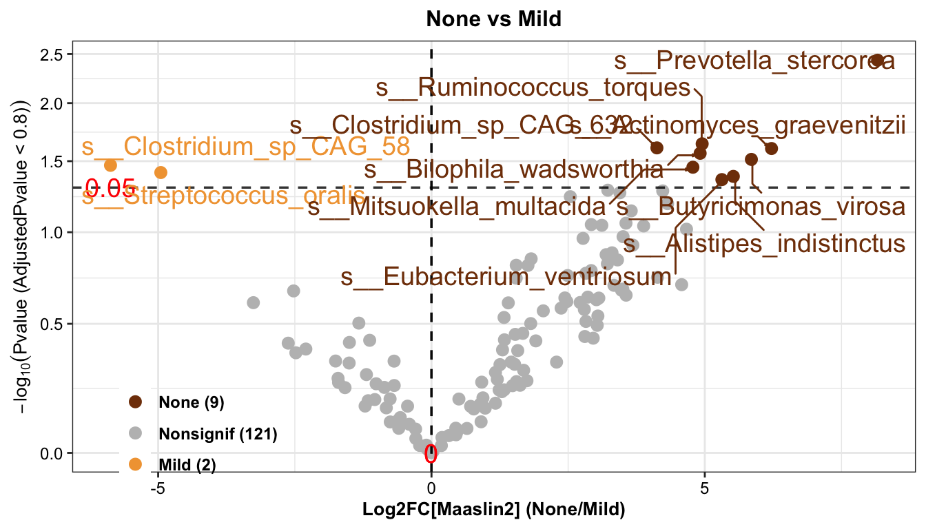
Result: 9 types of differential bacteria were enriched in the None group and 2 types of differential bacteria were enriched in the Mild group.
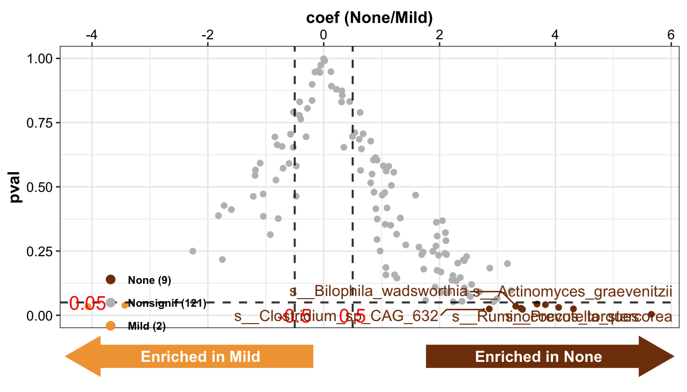
It is also recommended to use MicrobiomeAnalysis’ built-in volcano plot plot_volcano function, which provides more parameters for visualizing volcano plots.
MicrobiomeAnalysis::plot_volcano(
  da_res = Maaslin2_df$test_res,
  group_names = lf_grp[c(1, 2)],
  x_index = "coef",
  x_index_cutoff = 0.5,
  y_index = "pval",
  y_index_cutoff = 0.05,
  topN = 5,
  group_colors = c(lf_col[1], "grey", lf_col[2]),
  add_enrich_arrow = TRUE)
- Boxplot showing the relative abundance of the specific bacteria
get_boxplot(
  ps = Maaslin2_df$ps,
  feature = "s__Ruminococcus_torques",
  group = "LiverFatClass",
  group_names = c("None", "Mild"),
  group_color = lf_col[c(1, 2)],
  pl_title = "Ruminococcus_torques",
  pos_cutoff = -0.002)
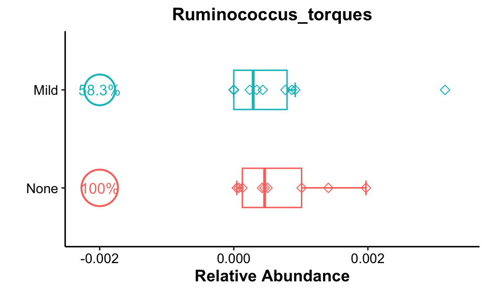
Result: Ruminococcus_torques was present at high rates in all None groups and its relative abundance was higher in the None group.
get_boxplot(
  ps = Maaslin2_df$ps,
  feature = "s__Streptococcus_oralis",
  group = "LiverFatClass",
  group_names = c("None", "Mild"),
  group_color = lf_col[c(1, 2)],
  pl_title = "Streptococcus_oralis",
  pos_cutoff = -0.002)
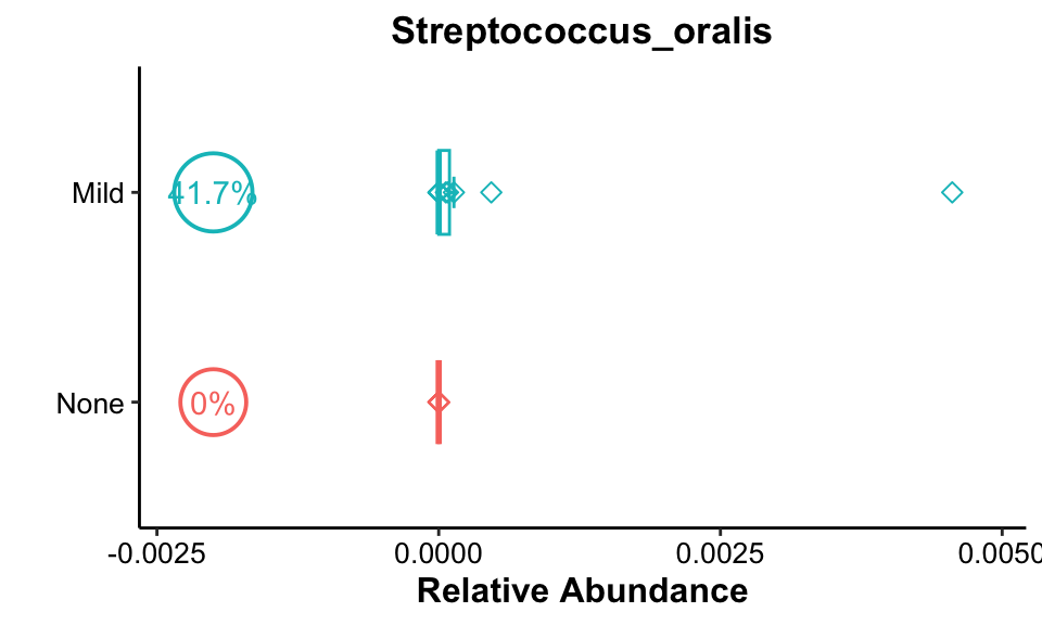
Result: Streptococcus_oralis was present at a high rate in both Mild groups and its relative abundance was higher in the Mild group.。
Analysis of Composition of Microbiomes with Bias Correction (ANCOM-BC)
Provide encapsulated function for calculation and plotting.
get_ANCOMBC: Obtaining the ANCOMBC result;
get_ANCOMBC_pl: Plotting the result.
get_ANCOMBC <- function(
  ps,
  taxa_level = c(NULL, "Phylum", "Class", "Order",
                 "Family", "Genus", "Species", "Strain"),
  filterCol = NULL,
  filterVars = NULL,
  group = c("LiverFatClass", "Gender"),
  group_names = c("None", "Mild", "Moderate", "Severe",
                  "Male", "Female"),
  prev_cutoff = 0.1,
  mean_threshold = 100,
  one_threshold = 1000,
  fix_vars = c("Age", "Gender")
  ) {

  # ps = phy_count
  # taxa_level = NULL
  # filterCol = NULL
  # filterVars = NULL
  # group = "LiverFatClass"
  # group_names = c("None", "Mild")
  # prev_cutoff = 0.1
  # mean_threshold = 100
  # one_threshold = 1000
  # fix_vars = c("Age", "Gender")


  if (!is.null(taxa_level)) {
    ps_taxa <- MicrobiomeAnalysis::aggregate_taxa(
      x = ps, level = taxa_level)
  } else {
    ps_taxa <- ps
  }

  metadata <- ps_taxa@sam_data %>%
    data.frame()

  if (is.null(filterCol)) {
    dat_cln <- metadata
  } else {
    colnames(metadata)[which(colnames(metadata) == filterCol)] <- "FiltCol"
    dat_cln <- metadata %>%
      dplyr::filter(FiltCol %in% filterVars)
    colnames(metadata)[which(colnames(metadata) == "FiltCol")] <- filterCol
  }

  # group for test
  dat_cln2 <- dat_cln
  colnames(dat_cln2)[which(colnames(dat_cln2) == group)] <- "Group_new"
  if (group_names[1] == "all") {
    dat_cln3 <- dat_cln2
  } else {
    dat_cln3 <- dat_cln2 %>%
      dplyr::filter(Group_new %in% group_names)
  }

  dat_cln3$Group_new <- factor(dat_cln3$Group_new, levels = group_names)
  colnames(dat_cln3)[which(colnames(dat_cln3) == "Group_new")] <- group

  ps_temp <- ps_taxa
  phyloseq::sample_data(ps_temp) <- phyloseq::sample_data(dat_cln3)

  # trim & filter
  ps_trim <- MicrobiomeAnalysis::trim_prevalence(
    object = ps_temp,
    cutoff = prev_cutoff,
    trim = "feature")
  ps_filter <- MicrobiomeAnalysis::filter_abundance(
    object = ps_trim,
    cutoff_mean = mean_threshold,
    cutoff_one = one_threshold)
  ps_filter <- ps_trim

  #################################################################
  # https://www.bioconductor.org/packages/release/bioc/vignettes/ANCOMBC/inst/doc/ANCOMBC.html

  fix_factors <- c(group, fix_vars)
  out <- ANCOMBC::ancombc(
    phyloseq = ps_filter,
    formula = paste(fix_factors, collapse = " + "),
    p_adj_method = "BH",
    prv_cut = 0.1,
    lib_cut = 0,
    group = group,
    struc_zero = TRUE,
    neg_lb = FALSE,
    tol = 1e-05,
    max_iter = 100,
    conserve = FALSE,
    alpha = 0.05,
    global = FALSE,
    n_cl = 1,
    verbose = FALSE)

  # Result from the ANCOM-BC log-linear model to determine taxa that are differentially abundant according to the covariate of interest.
  # It contains: 1) log fold changes; 2) standard errors;
  # 3) test statistics; 4) p-values; 5) adjusted p-values;
  # 6) indicators whether the taxon is differentially abundant (TRUE) or not (FALSE)

  res_list <- out$res
  res_temp <- cbind(res_list$lfc$taxon,
                    res_list$lfc[3],
                    res_list$se[3],
                    res_list$W[3],
                    res_list$p_val[3],
                    res_list$q_val[3],
                    res_list$diff_abn[3]) %>%
    setNames(c("feature", "lfc", "se", "W", "p_val", "q_val", "diff_abu"))

  # Number of Group
  input_metadata <- phyloseq::sample_data(ps_filter) %>%
    data.frame()
  colnames(input_metadata)[which(colnames(input_metadata) == group)] <- "Compvar"
  dat_status <- table(input_metadata$Compvar)
  dat_status_number <- as.numeric(dat_status)
  dat_status_name <- names(dat_status)
  res_temp$Block <- paste(paste(dat_status_number[1], dat_status_name[1], sep = "_"),
                       "vs",
                       paste(dat_status_number[2], dat_status_name[2], sep = "_"))
  res_test <- res_temp %>%
    dplyr::select(feature, Block, everything()) %>%
    dplyr::inner_join(ps_filter@tax_table %>%
                        data.frame() %>%
                        tibble::rownames_to_column("feature"),
                      by = "feature") %>%
    dplyr::rename(TaxaID = feature) %>%
    dplyr::mutate(Enrichment = ifelse(as.numeric(lfc) > 0, group_names[2], group_names[1])) %>%
    dplyr::select(TaxaID, Block, lfc, Enrichment, everything())

  # final results list
  res <- list(ps = ps_filter,
              test_res = res_test)

  return(res)
}

# plot
get_ANCOMBC_pl <- function(
    dat,
    lg2fc_cutoff = 0,
    pval_cutoff = 0.05,
    qval_cutoff = 0.8, #0.05,
    group_color,
    plot_title) {

  # group_names
  group_names <- gsub("\\d+_", "", unlist(strsplit(dat$Block[1], " vs ")))

  dat$lg2fc <- dat$lfc
  dat$pval <- dat$p_val
  dat$qval <- dat$q_val

  # enrichment by beta and Pvalue AdjustedPvalue
  dat[which(dat$lg2fc > lg2fc_cutoff &
              dat$pval < pval_cutoff &
              dat$qval < qval_cutoff),
      "EnrichedDir"] <- group_names[2]
  dat[which(dat$lg2fc < -lg2fc_cutoff &
              dat$pval < pval_cutoff &
              dat$qval < qval_cutoff),
      "EnrichedDir"] <- group_names[1]
  dat[which(abs(dat$lg2fc) <= lg2fc_cutoff |
              dat$pval >= pval_cutoff |
              dat$qval >= qval_cutoff),
      "EnrichedDir"] <- "Nonsignif"

  dat$EnrichedDir <- factor(dat$EnrichedDir,
                            levels = c(group_names[2], "Nonsignif", group_names[1]))

  # dat status
  df_status <- table(dat$EnrichedDir) %>%
    data.frame() %>%
    stats::setNames(c("Group", "Number"))
  grp1_number <- with(df_status, df_status[Group %in% group_names[2], "Number"])
  grp2_number <- with(df_status, df_status[Group %in% group_names[1], "Number"])
  nsf_number <- with(df_status, df_status[Group %in% "Nonsignif", "Number"])
  legend_label <- c(paste0(group_names[2], " (", grp1_number, ")"),
                    paste0("Nonsignif", " (", nsf_number, ")"),
                    paste0(group_names[1], " (", grp2_number, ")"))

  # significant features
  dat_signif <- dat %>%
    dplyr::arrange(lg2fc, pval, qval) %>%
    dplyr::filter(pval < pval_cutoff) %>%
    dplyr::filter(qval < qval_cutoff) %>%
    dplyr::filter(abs(lg2fc) > lg2fc_cutoff)

  # color
  plot_group_color <- c(group_color[1], "grey", group_color[2])
  names(plot_group_color) <- c(group_names[1], "Nonsignif", group_names[2])

  # labels
  xlabel <- paste0("Log2FC[ANCOMBC] (", paste(rev(group_names), collapse = "/"), ")")
  ylable <- expression(-log[10]("Pvalue (AdjustedPvalue < 0.25)"))


  pl <- ggplot(dat, aes(x = lg2fc, y = -log10(pval), color = EnrichedDir)) +
    geom_point(size = 2, alpha = 1, stroke = 1) +
    scale_color_manual(name = NULL,
                       values = plot_group_color,
                       labels = legend_label) +
    xlab(xlabel) +
    ylab(ylable) +
    geom_vline(xintercept = lg2fc_cutoff, alpha = .8, linetype = 2, size = 0.6) +
    geom_vline(xintercept = -lg2fc_cutoff, alpha = .8, linetype = 2, size = 0.6) +
    annotate("text",
             x = lg2fc_cutoff, y = 0,
             label = lg2fc_cutoff,
             size = 5, color = "red") +
    annotate("text", x = -lg2fc_cutoff, y = 0,
             label = -lg2fc_cutoff,
             size = 5, color = "red") +
    guides(color = guide_legend(override.aes = list(size = 2))) +
    scale_y_continuous(trans = "log1p") +
    geom_hline(yintercept = -log10(pval_cutoff), alpha = .8, linetype = 2, size = 0.6) +
    annotate("text",
             x = min(dat$lg2fc),
             y = -log10(pval_cutoff),
             label = pval_cutoff,
             size = 5, color = "red") +
    ggrepel::geom_text_repel(data = dat_signif,
                             aes(label = TaxaID),
                             size = 5,
                             max.overlaps = getOption("ggrepel.max.overlaps", default = 80),
                             segment.linetype = 1,
                             segment.curvature = -1e-20,
                             box.padding = unit(0.35, "lines"),
                             point.padding = unit(0.3, "lines"),
                             arrow = arrow(length = unit(0.005, "npc")),
                             bg.r = 0.15) +
    theme_bw() +
    theme(axis.title = element_text(size = 10, face = "bold", color = "black"),
          axis.text = element_text(size = 9, color = "black"),
          text = element_text(size = 8, color = "black"),
          legend.position = c(.15, .1),
          legend.key.height = unit(0.6, "cm"),
          legend.text = element_text(size = 9, face = "bold", color = "black"),
          strip.text = element_text(size = 8, face = "bold"),
          legend.background = element_rect(fill = rgb(1, 1, 1, alpha = 0.001), color = NA)) + # legend background transparency
    ggtitle(plot_title) +
    theme(plot.title = element_text(face = "bold", size = 12, hjust = .5))

  return(pl)
}
- Differential Analysis from ANCOMBC
Using LiverFatClass as the comparison group, two subgroups, None and Mild, were selected for difference analysis.
ANCOMBC_df <- get_ANCOMBC(
  ps = phy_count,
  taxa_level = NULL,
  filterCol = NULL,
  filterVars = NULL,
  group = "LiverFatClass",
  group_names = c("None", "Mild"),
  prev_cutoff = 0.1,
  mean_threshold = 100,
  one_threshold = 1000,
  fix_vars = c("Age", "Gender"))


head(ANCOMBC_df$test_res[, 1:3], 5)
##                            TaxaID             Block         lfc
## 1     s__Actinomyces_graevenitzii 9_None vs 12_Mild -0.69410607
## 2    s__Actinomyces_odontolyticus 9_None vs 12_Mild  0.07148274
## 3         s__Actinomyces_sp_ICM47 9_None vs 12_Mild  1.80267320
## 4 s__Bifidobacterium_adolescentis 9_None vs 12_Mild -1.83673365
## 5    s__Bifidobacterium_angulatum 9_None vs 12_Mild  2.10805876
Result: The corrected pval, also known as qval, were all greater than 0.05, and no differential species were screened; a qvalue threshold of 0.25 was used in the lower panel in order to visualize the results.
- Visualization
ANCOMBC_pl <- get_ANCOMBC_pl(
  dat = ANCOMBC_df$test_res,
  lg2fc_cutoff = 0,
  pval_cutoff = 0.05,
  qval_cutoff = 0.25,
  group_color = lf_col[c(1, 2)],
  plot_title = "None vs Mild")

ANCOMBC_pl
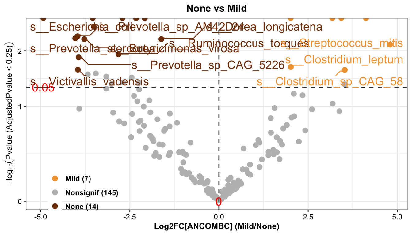
Result: 14 types of differential bacteria were enriched in the None group and 7 types of differential bacteria were enriched in the Mild group.
- Boxplot showing the relative abundance of the specific bacteria
get_boxplot(
  ps = ANCOMBC_df$ps,
  feature = "s__Clostridium_leptum",
  group = "LiverFatClass",
  group_names = c("None", "Mild"),
  group_color = lf_col[c(1, 2)],
  pl_title = "Clostridium_leptum",
  pos_cutoff = -200)
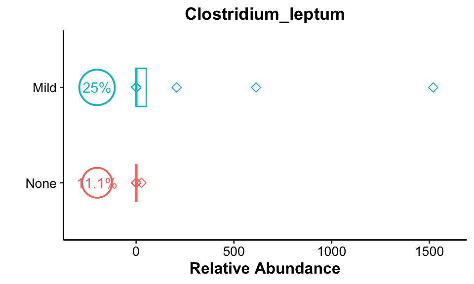
Result: Clostridium_leptum had high occurrences in both Mild groups, and relative abundance was higher in the Mild group.
Consolidataion of the above results
The results of lefse were used as a benchmark to combine the results of the three analytical methods mentioned above.
get_mergeRes <- function(
    DA1,
    DA2,
    DA3,
    lg2fc_cutoff = 0,
    pval_cutoff = 0.05,
    qval_cutoff = 0.3,
    group_colors) {

  # DA1 = lefse_df$test_res
  # DA2 = Maaslin2_df$test_res
  # DA3 = ANCOMBC_df$test_res
  # lg2fc_cutoff = 0
  # pval_cutoff = 0.05
  # qval_cutoff = 0.8
  # group_colors = lf_col[c(1, 2)]

  # group_names
  group_names <- gsub("\\d+_", "", unlist(strsplit(DA1$Block[1], " vs ")))

  DA_lefse_cln <- DA1 %>%
    dplyr::select(TaxaID, Block, LDA_Score, Enrichment,
                  Kingdom, Phylum, Genus, Species) %>%
    dplyr::rename(Lefse_Enrichment = Enrichment)

  DA_maaslin2_cln <- DA2 %>%
    dplyr::select(TaxaID, coef, Enrichment,
                  pval, qval) %>%
    dplyr::mutate(lg2fc = log2(exp(coef))) %>%
    dplyr::rename(Maaslin2_Enrichment = Enrichment,
                  Maaslin2_pval = pval,
                  Maaslin2_qval = qval,
                  Maaslin2_lg2fc = lg2fc)
  DA_maaslin2_cln[which(DA_maaslin2_cln$Maaslin2_lg2fc > lg2fc_cutoff &
            DA_maaslin2_cln$Maaslin2_pval < pval_cutoff &
            DA_maaslin2_cln$Maaslin2_qval < qval_cutoff),
      "Maaslin2_Enrichment"] <- group_names[2]
  DA_maaslin2_cln[which(DA_maaslin2_cln$Maaslin2_lg2fc < -lg2fc_cutoff &
            DA_maaslin2_cln$Maaslin2_pval < pval_cutoff &
            DA_maaslin2_cln$Maaslin2_qval < qval_cutoff),
      "Maaslin2_Enrichment"] <- group_names[1]
  DA_maaslin2_cln[which(abs(DA_maaslin2_cln$Maaslin2_lg2fc) <= lg2fc_cutoff |
            DA_maaslin2_cln$Maaslin2_pval >= pval_cutoff |
            DA_maaslin2_cln$Maaslin2_qval >= qval_cutoff),
      "Maaslin2_Enrichment"] <- "Nonsignif"

  DA_ANCOMBC_cln <- DA3 %>%
    dplyr::select(TaxaID, lfc, Enrichment,
                  p_val, q_val) %>%
    dplyr::rename(ANCOMBC_Enrichment = Enrichment,
                  ANCOMBC_pval = p_val,
                  ANCOMBC_qval = q_val,
                  ANCOMBC_lg2fc = lfc)
  DA_ANCOMBC_cln[which(DA_ANCOMBC_cln$ANCOMBC_lg2fc > lg2fc_cutoff &
            DA_ANCOMBC_cln$ANCOMBC_pval < pval_cutoff &
            DA_ANCOMBC_cln$ANCOMBC_qval < qval_cutoff),
      "ANCOMBC_Enrichment"] <- group_names[2]
  DA_ANCOMBC_cln[which(DA_ANCOMBC_cln$ANCOMBC_lg2fc < -lg2fc_cutoff &
            DA_ANCOMBC_cln$ANCOMBC_pval < pval_cutoff &
            DA_ANCOMBC_cln$ANCOMBC_qval < qval_cutoff),
      "ANCOMBC_Enrichment"] <- group_names[1]
  DA_ANCOMBC_cln[which(abs(DA_ANCOMBC_cln$ANCOMBC_lg2fc) <= lg2fc_cutoff |
            DA_ANCOMBC_cln$ANCOMBC_pval >= pval_cutoff |
            DA_ANCOMBC_cln$ANCOMBC_qval >= qval_cutoff),
      "ANCOMBC_Enrichment"] <- "Nonsignif"

  res <- DA_lefse_cln %>%
    dplyr::left_join(DA_maaslin2_cln,
                      by = "TaxaID") %>%
    dplyr::left_join(DA_ANCOMBC_cln,
                      by = "TaxaID") %>%
    dplyr::select(TaxaID, Block, LDA_Score, Lefse_Enrichment,
                  Maaslin2_Enrichment, coef, Maaslin2_lg2fc, Maaslin2_pval, Maaslin2_qval,
                  ANCOMBC_Enrichment, ANCOMBC_lg2fc, ANCOMBC_pval, ANCOMBC_qval,
                  Kingdom, Phylum, Genus, Species) %>%
    dplyr::group_by(TaxaID) %>%
    dplyr::mutate(Signif = ifelse(
      all(Maaslin2_Enrichment != "Nonsignif",
          ANCOMBC_Enrichment != "Nonsignif"), "+",
      ifelse(Maaslin2_Enrichment != "Nonsignif", "*",
        ifelse(ANCOMBC_Enrichment != "Nonsignif", "#", "")))) %>%

    # dplyr::mutate(Signif = ifelse(Maaslin2_Enrichment != "Nonsignif", "*",
    #                               ifelse(ANCOMBC_Enrichment != "Nonsignif", "#",
    #                                      ifelse(all(Maaslin2_Enrichment != "Nonsignif",
    #                                                 ANCOMBC_Enrichment != "Nonsignif"),
    #                                             "+", "")))) %>%
    dplyr::ungroup()

  if (length(grep("^t__", res$TaxaID)) > 1) {
    plotdata <- res %>%
      dplyr::group_by(TaxaID) %>%
      dplyr::mutate(TaxaID = gsub("t__", "", TaxaID)) %>%
      dplyr::ungroup() %>%
      dplyr::mutate(FeatureID = paste0(TaxaID, " (", Species, ")")) %>%
      dplyr::select(FeatureID, LDA_Score, Lefse_Enrichment, Signif, Phylum) %>%
      dplyr::mutate(Lefse_Enrichment = factor(Lefse_Enrichment, levels = group_names)) %>%
      dplyr::mutate(
        FeatureID = factor(FeatureID, levels = FeatureID[order(LDA_Score, decreasing = TRUE)]),
        label_y = ifelse(LDA_Score < 0, 0.2, -0.2),
        label_hjust = ifelse(LDA_Score < 0, 0, 1),
        label_hjust2 = ifelse(LDA_Score > 0, 0, 1))
  } else {
    plotdata <- res %>%
      dplyr::mutate(FeatureID = TaxaID) %>%
      dplyr::select(FeatureID, LDA_Score, Lefse_Enrichment, Signif, Phylum) %>%
      dplyr::mutate(Lefse_Enrichment = factor(Lefse_Enrichment, levels = group_names)) %>%
      dplyr::mutate(
        FeatureID = factor(FeatureID, levels = FeatureID[order(LDA_Score, decreasing = TRUE)]),
        label_y = ifelse(LDA_Score < 0, 0.2, -0.2),
        label_hjust = ifelse(LDA_Score < 0, 0, 1),
        label_hjust2 = ifelse(LDA_Score > 0, 0, 1))
  }

  if (length(grep("unclassified", plotdata$Phylum)) > 0) {
    plotdata <- plotdata[-grep("unclassified", plotdata$Phylum), , ] %>%
      dplyr::mutate(Phylum = gsub("p__", "", Phylum))
  } else {
    plotdata <- plotdata %>%
      dplyr::mutate(Phylum = gsub("p__", "", Phylum))
  }

  plotdata$Phylum <- factor(plotdata$Phylum, levels = unique(plotdata$Phylum))
  phylum_colors <- RColorBrewer::brewer.pal(n = length(levels(plotdata$Phylum)),
                                            name = "Dark2")

  pl <- ggplot(plotdata, aes(x = FeatureID, y = LDA_Score, fill = Lefse_Enrichment)) +
    geom_bar(stat = "identity", color = "white") +
    geom_text(aes(y = label_y, label = FeatureID, hjust = label_hjust, color = Phylum), fontface = "italic") +
    geom_text(aes(y = LDA_Score, label = Signif, hjust = label_hjust2), size = 6) +
    coord_flip() +
    scale_y_continuous(expression(log[10](italic("LDA score"))),
                       breaks = -4:4, limits = c(-5, 5)) +
    scale_fill_manual(name = NULL, values = group_colors) +
    scale_color_manual(name = "Phylum", values = phylum_colors) +
    guides(fill = guide_legend(order = 1),
           color = guide_legend(order = 2)) +
    theme_minimal() +
    theme(axis.text.y = element_blank(),
          axis.ticks.y = element_blank(),
          axis.title.y = element_blank(),
          legend.position = "right",
          legend.justification = 0.5,
          panel.grid.major.y = element_blank(),
          panel.grid.minor.y = element_blank(),
          panel.grid.major.x = element_line(color = "grey80", linetype = "dashed"),
          panel.grid.minor.x = element_blank())

  return(pl)
}


Merge_DA_pl <- get_mergeRes(
  DA1 = lefse_df$test_res,
  DA2 = Maaslin2_df$test_res,
  DA3 = ANCOMBC_df$test_res,
  lg2fc_cutoff = 0,
  pval_cutoff = 0.05,
  qval_cutoff = 0.8,
  group_colors = lf_col[c(1, 2)])

Merge_DA_pl
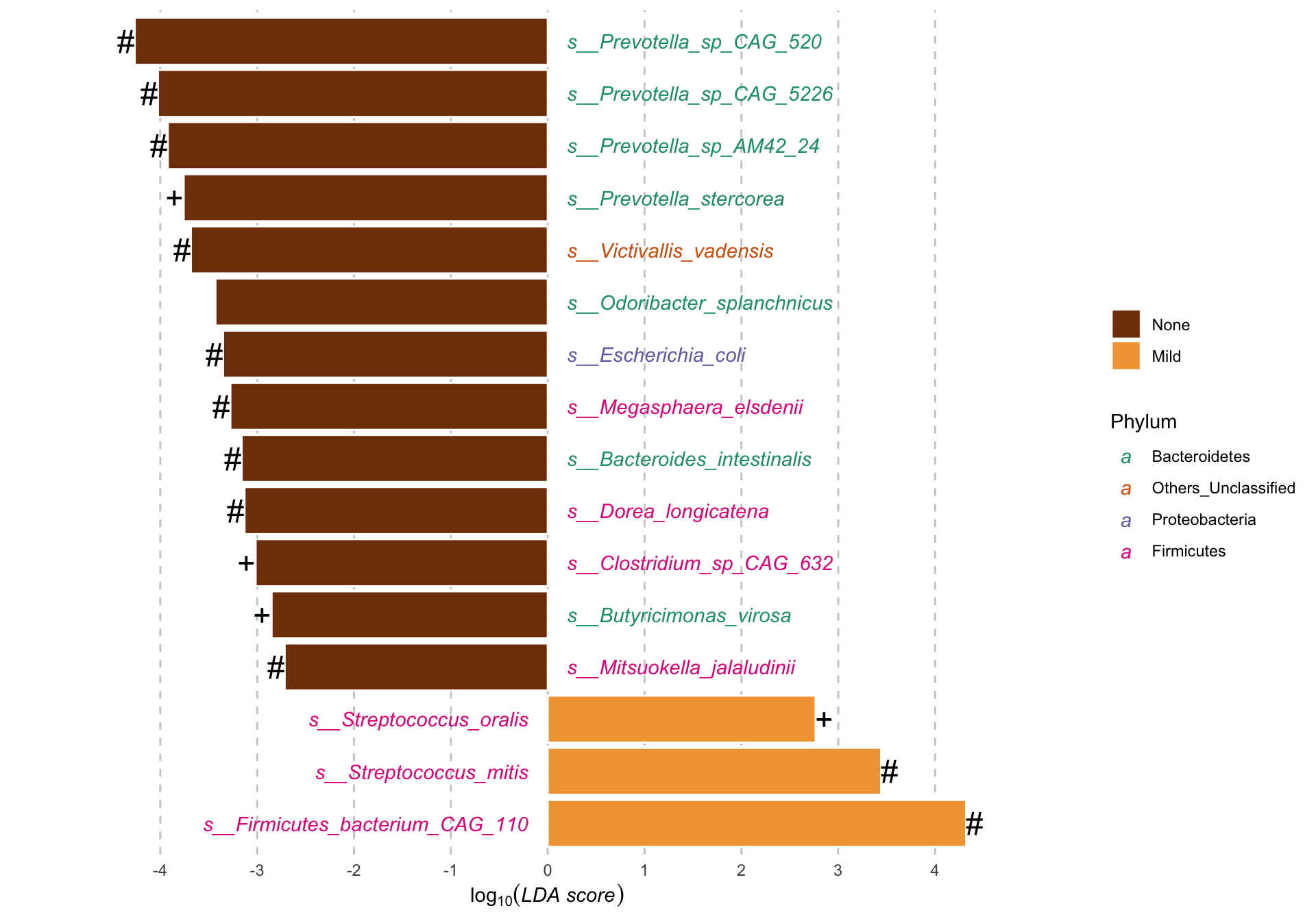
Results:
Differential abundance of metagenomic species measured by linear discriminant analysis of effect size (LefSe) according to the LiverFatClass group.
LDA; Linear discriminant analysis.
+ Multivariate analysis (ANCOM-BC & Maaslin2) with a false discovery rate (FDR) adjusted p-value < 0.8.
* Multivariate analysis (Maaslin2) with a false discovery rate (FDR) adjusted p-value < 0.8.
# Multivariate analysis (ANCOM-BC) with a false discovery rate (FDR) adjusted p-value < 0.8.
Conclusion
There were relatively high overlap of differential microbiota identified by the three different approaches when using LefSe as a benchmark.
Of the three difference methods, the Maaslin2 method was relatively the most stringent and screened for fewer difference species, whereas LefSe and ANCOM-BC screened for more species. LefSe did not take into account multiple test correction, and ANCOM-BC used zero inflation as well as correcting for between-sample variation methods, which resulted in more difference species being identified. It is important to note that, as can be seen from the boxplots of individual species later on, strict filtering of species occurrence is required, which can prevent low occurrence species from being identified (by choosing the appropriate filtering parameters according to the purpose of the study).
Session info
devtools::session_info()
## ─ Session info ───────────────────────────────────────────────────────────────
## setting value
## version R version 4.3.1 (2023-06-16)
## os macOS Monterey 12.2.1
## system x86_64, darwin20
## ui X11
## language (EN)
## collate en_US.UTF-8
## ctype en_US.UTF-8
## tz Asia/Shanghai
## date 2024-02-07
## pandoc 3.1.3 @ /Users/zouhua/opt/anaconda3/bin/ (via rmarkdown)
##
## ─ Packages ───────────────────────────────────────────────────────────────────
## package * version date (UTC) lib source
## abind 1.4-5 2016-07-21 [1] CRAN (R 4.3.0)
## ade4 1.7-22 2023-02-06 [1] CRAN (R 4.3.0)
## ANCOMBC * 2.4.0 2023-10-24 [1] Bioconductor
## ape 5.7-1 2023-03-13 [1] CRAN (R 4.3.0)
## backports 1.4.1 2021-12-13 [1] CRAN (R 4.3.0)
## base64enc 0.1-3 2015-07-28 [1] CRAN (R 4.3.0)
## beachmat 2.18.0 2023-10-24 [1] Bioconductor
## beeswarm 0.4.0 2021-06-01 [1] CRAN (R 4.3.0)
## biglm 0.9-2.1 2020-11-27 [1] CRAN (R 4.3.0)
## Biobase 2.62.0 2023-10-24 [1] Bioconductor
## BiocGenerics 0.48.1 2023-11-01 [1] Bioconductor
## BiocNeighbors 1.20.2 2024-01-07 [1] Bioconductor 3.18 (R 4.3.2)
## BiocParallel 1.36.0 2023-10-24 [1] Bioconductor
## BiocSingular 1.18.0 2023-10-24 [1] Bioconductor
## biomformat 1.30.0 2023-10-24 [1] Bioconductor
## Biostrings 2.70.2 2024-01-28 [1] Bioconductor 3.18 (R 4.3.2)
## bit 4.0.5 2022-11-15 [1] CRAN (R 4.3.0)
## bit64 4.0.5 2020-08-30 [1] CRAN (R 4.3.0)
## bitops 1.0-7 2021-04-24 [1] CRAN (R 4.3.0)
## blob 1.2.4 2023-03-17 [1] CRAN (R 4.3.0)
## blogdown 1.19 2024-02-01 [1] CRAN (R 4.3.2)
## bluster 1.12.0 2023-10-24 [1] Bioconductor
## bookdown 0.37 2023-12-01 [1] CRAN (R 4.3.0)
## boot 1.3-28.1 2022-11-22 [1] CRAN (R 4.3.1)
## broom 1.0.5 2023-06-09 [1] CRAN (R 4.3.0)
## bslib 0.6.1 2023-11-28 [1] CRAN (R 4.3.0)
## cachem 1.0.8 2023-05-01 [1] CRAN (R 4.3.0)
## car 3.1-2 2023-03-30 [1] CRAN (R 4.3.0)
## carData 3.0-5 2022-01-06 [1] CRAN (R 4.3.0)
## caTools 1.18.2 2021-03-28 [1] CRAN (R 4.3.0)
## cellranger 1.1.0 2016-07-27 [1] CRAN (R 4.3.0)
## checkmate 2.3.1 2023-12-04 [1] CRAN (R 4.3.0)
## class 7.3-22 2023-05-03 [1] CRAN (R 4.3.1)
## cli 3.6.2 2023-12-11 [1] CRAN (R 4.3.0)
## cluster 2.1.4 2022-08-22 [1] CRAN (R 4.3.1)
## codetools 0.2-19 2023-02-01 [1] CRAN (R 4.3.1)
## colorspace 2.1-0 2023-01-23 [1] CRAN (R 4.3.0)
## cowplot 1.1.3 2024-01-22 [1] CRAN (R 4.3.2)
## crayon 1.5.2 2022-09-29 [1] CRAN (R 4.3.0)
## curl 5.2.0 2023-12-08 [1] CRAN (R 4.3.0)
## CVXR 1.0-12 2024-02-02 [1] CRAN (R 4.3.2)
## data.table 1.15.0 2024-01-30 [1] CRAN (R 4.3.2)
## DBI 1.2.1 2024-01-12 [1] CRAN (R 4.3.0)
## DECIPHER 2.30.0 2023-10-24 [1] Bioconductor
## decontam 1.22.0 2023-10-24 [1] Bioconductor
## DelayedArray 0.28.0 2023-10-24 [1] Bioconductor
## DelayedMatrixStats 1.24.0 2023-10-24 [1] Bioconductor
## DEoptimR 1.1-3 2023-10-07 [1] CRAN (R 4.3.0)
## DescTools 0.99.54 2024-02-03 [1] CRAN (R 4.3.2)
## DESeq2 1.42.0 2023-10-24 [1] Bioconductor
## devtools 2.4.5 2022-10-11 [1] CRAN (R 4.3.0)
## digest 0.6.34 2024-01-11 [1] CRAN (R 4.3.0)
## DirichletMultinomial 1.44.0 2023-10-24 [1] Bioconductor
## doParallel 1.0.17 2022-02-07 [1] CRAN (R 4.3.0)
## doRNG * 1.8.6 2023-01-16 [1] CRAN (R 4.3.0)
## dplyr * 1.1.4 2023-11-17 [1] CRAN (R 4.3.0)
## e1071 1.7-14 2023-12-06 [1] CRAN (R 4.3.0)
## ellipsis 0.3.2 2021-04-29 [1] CRAN (R 4.3.0)
## energy 1.7-11 2022-12-22 [1] CRAN (R 4.3.0)
## evaluate 0.23 2023-11-01 [1] CRAN (R 4.3.0)
## Exact 3.2 2022-09-25 [1] CRAN (R 4.3.0)
## expm 0.999-9 2024-01-11 [1] CRAN (R 4.3.0)
## fansi 1.0.6 2023-12-08 [1] CRAN (R 4.3.0)
## farver 2.1.1 2022-07-06 [1] CRAN (R 4.3.0)
## fastmap 1.1.1 2023-02-24 [1] CRAN (R 4.3.0)
## forcats * 1.0.0 2023-01-29 [1] CRAN (R 4.3.0)
## foreach * 1.5.2 2022-02-02 [1] CRAN (R 4.3.0)
## foreign 0.8-84 2022-12-06 [1] CRAN (R 4.3.1)
## Formula 1.2-5 2023-02-24 [1] CRAN (R 4.3.0)
## fs 1.6.3 2023-07-20 [1] CRAN (R 4.3.0)
## generics 0.1.3 2022-07-05 [1] CRAN (R 4.3.0)
## GenomeInfoDb 1.38.5 2023-12-28 [1] Bioconductor 3.18 (R 4.3.2)
## GenomeInfoDbData 1.2.11 2024-01-24 [1] Bioconductor
## GenomicRanges 1.54.1 2023-10-29 [1] Bioconductor
## getopt 1.20.4 2023-10-01 [1] CRAN (R 4.3.0)
## ggbeeswarm 0.7.2 2023-04-29 [1] CRAN (R 4.3.0)
## ggplot2 * 3.4.4 2023-10-12 [1] CRAN (R 4.3.0)
## ggpubr * 0.6.0 2023-02-10 [1] CRAN (R 4.3.0)
## ggrepel 0.9.5 2024-01-10 [1] CRAN (R 4.3.0)
## ggsignif 0.6.4 2022-10-13 [1] CRAN (R 4.3.0)
## gld 2.6.6 2022-10-23 [1] CRAN (R 4.3.0)
## glmnet 4.1-8 2023-08-22 [1] CRAN (R 4.3.0)
## glue 1.7.0 2024-01-09 [1] CRAN (R 4.3.0)
## gmp 0.7-4 2024-01-15 [1] CRAN (R 4.3.0)
## gplots 3.1.3.1 2024-02-02 [1] CRAN (R 4.3.2)
## gridExtra 2.3 2017-09-09 [1] CRAN (R 4.3.0)
## gsl 2.1-8 2023-01-24 [1] CRAN (R 4.3.0)
## gtable 0.3.4 2023-08-21 [1] CRAN (R 4.3.0)
## gtools 3.9.5 2023-11-20 [1] CRAN (R 4.3.0)
## hash 2.2.6.3 2023-08-19 [1] CRAN (R 4.3.0)
## highr 0.10 2022-12-22 [1] CRAN (R 4.3.0)
## Hmisc 5.1-1 2023-09-12 [1] CRAN (R 4.3.0)
## hms 1.1.3 2023-03-21 [1] CRAN (R 4.3.0)
## htmlTable 2.4.2 2023-10-29 [1] CRAN (R 4.3.0)
## htmltools 0.5.7 2023-11-03 [1] CRAN (R 4.3.0)
## htmlwidgets 1.6.4 2023-12-06 [1] CRAN (R 4.3.0)
## httpuv 1.6.14 2024-01-26 [1] CRAN (R 4.3.2)
## httr 1.4.7 2023-08-15 [1] CRAN (R 4.3.0)
## igraph 2.0.1.1 2024-01-30 [1] CRAN (R 4.3.2)
## IRanges 2.36.0 2023-10-24 [1] Bioconductor
## irlba 2.3.5.1 2022-10-03 [1] CRAN (R 4.3.0)
## iterators 1.0.14 2022-02-05 [1] CRAN (R 4.3.0)
## jquerylib 0.1.4 2021-04-26 [1] CRAN (R 4.3.0)
## jsonlite 1.8.8 2023-12-04 [1] CRAN (R 4.3.0)
## KernSmooth 2.23-21 2023-05-03 [1] CRAN (R 4.3.1)
## knitr 1.45 2023-10-30 [1] CRAN (R 4.3.0)
## labeling 0.4.3 2023-08-29 [1] CRAN (R 4.3.0)
## later 1.3.2 2023-12-06 [1] CRAN (R 4.3.0)
## lattice 0.21-8 2023-04-05 [1] CRAN (R 4.3.1)
## lazyeval 0.2.2 2019-03-15 [1] CRAN (R 4.3.0)
## lifecycle 1.0.4 2023-11-07 [1] CRAN (R 4.3.0)
## limma 3.58.1 2023-10-31 [1] Bioconductor
## lme4 1.1-35.1 2023-11-05 [1] CRAN (R 4.3.0)
## lmerTest 3.1-3 2020-10-23 [1] CRAN (R 4.3.0)
## lmom 3.0 2023-08-29 [1] CRAN (R 4.3.0)
## locfit 1.5-9.8 2023-06-11 [1] CRAN (R 4.3.0)
## logging 0.10-108 2019-07-14 [1] CRAN (R 4.3.0)
## lpsymphony 1.30.0 2023-10-24 [1] Bioconductor (R 4.3.1)
## lubridate * 1.9.3 2023-09-27 [1] CRAN (R 4.3.0)
## Maaslin2 * 1.7.3 2024-01-24 [1] Bioconductor
## magrittr 2.0.3 2022-03-30 [1] CRAN (R 4.3.0)
## MASS 7.3-60 2023-05-04 [1] CRAN (R 4.3.1)
## Matrix 1.6-5 2024-01-11 [1] CRAN (R 4.3.0)
## MatrixGenerics 1.14.0 2023-10-24 [1] Bioconductor
## matrixStats 1.2.0 2023-12-11 [1] CRAN (R 4.3.0)
## memoise 2.0.1 2021-11-26 [1] CRAN (R 4.3.0)
## metagenomeSeq 1.43.0 2023-04-25 [1] Bioconductor
## mgcv 1.8-42 2023-03-02 [1] CRAN (R 4.3.1)
## mia 1.10.0 2023-10-24 [1] Bioconductor
## MicrobiomeAnalysis * 1.0.3 2024-02-06 [1] Github (HuaZou/MicrobiomeAnalysis@fd2a6a2)
## mime 0.12 2021-09-28 [1] CRAN (R 4.3.0)
## miniUI 0.1.1.1 2018-05-18 [1] CRAN (R 4.3.0)
## minqa 1.2.6 2023-09-11 [1] CRAN (R 4.3.0)
## multcomp 1.4-25 2023-06-20 [1] CRAN (R 4.3.0)
## MultiAssayExperiment 1.28.0 2023-10-24 [1] Bioconductor
## multtest 2.58.0 2023-10-24 [1] Bioconductor
## munsell 0.5.0 2018-06-12 [1] CRAN (R 4.3.0)
## mvtnorm 1.2-4 2023-11-27 [1] CRAN (R 4.3.0)
## nlme 3.1-162 2023-01-31 [1] CRAN (R 4.3.1)
## nloptr 2.0.3 2022-05-26 [1] CRAN (R 4.3.0)
## nnet 7.3-19 2023-05-03 [1] CRAN (R 4.3.1)
## numDeriv 2016.8-1.1 2019-06-06 [1] CRAN (R 4.3.0)
## optparse 1.7.4 2024-01-16 [1] CRAN (R 4.3.0)
## pbapply 1.7-2 2023-06-27 [1] CRAN (R 4.3.0)
## pcaPP 2.0-4 2023-12-07 [1] CRAN (R 4.3.0)
## permute 0.9-7 2022-01-27 [1] CRAN (R 4.3.0)
## phyloseq * 1.46.0 2023-10-24 [1] Bioconductor
## pillar 1.9.0 2023-03-22 [1] CRAN (R 4.3.0)
## pkgbuild 1.4.3 2023-12-10 [1] CRAN (R 4.3.0)
## pkgconfig 2.0.3 2019-09-22 [1] CRAN (R 4.3.0)
## pkgload 1.3.4 2024-01-16 [1] CRAN (R 4.3.0)
## plyr 1.8.9 2023-10-02 [1] CRAN (R 4.3.0)
## profvis 0.3.8 2023-05-02 [1] CRAN (R 4.3.0)
## promises 1.2.1 2023-08-10 [1] CRAN (R 4.3.0)
## proxy 0.4-27 2022-06-09 [1] CRAN (R 4.3.0)
## purrr * 1.0.2 2023-08-10 [1] CRAN (R 4.3.0)
## R6 2.5.1 2021-08-19 [1] CRAN (R 4.3.0)
## rbibutils 2.2.16 2023-10-25 [1] CRAN (R 4.3.0)
## RColorBrewer 1.1-3 2022-04-03 [1] CRAN (R 4.3.0)
## Rcpp 1.0.12 2024-01-09 [1] CRAN (R 4.3.0)
## RCurl 1.98-1.14 2024-01-09 [1] CRAN (R 4.3.0)
## Rdpack 2.6 2023-11-08 [1] CRAN (R 4.3.0)
## readr * 2.1.5 2024-01-10 [1] CRAN (R 4.3.0)
## readxl 1.4.3 2023-07-06 [1] CRAN (R 4.3.0)
## remotes 2.4.2.1 2023-07-18 [1] CRAN (R 4.3.0)
## reshape2 1.4.4 2020-04-09 [1] CRAN (R 4.3.0)
## rhdf5 2.46.1 2023-11-29 [1] Bioconductor
## rhdf5filters 1.14.1 2023-11-06 [1] Bioconductor
## Rhdf5lib 1.24.1 2023-12-12 [1] Bioconductor 3.18 (R 4.3.2)
## rlang 1.1.3 2024-01-10 [1] CRAN (R 4.3.0)
## rmarkdown 2.25 2023-09-18 [1] CRAN (R 4.3.0)
## Rmpfr 0.9-5 2024-01-21 [1] CRAN (R 4.3.0)
## rngtools * 1.5.2 2021-09-20 [1] CRAN (R 4.3.0)
## robustbase 0.99-1 2023-11-29 [1] CRAN (R 4.3.0)
## rootSolve 1.8.2.4 2023-09-21 [1] CRAN (R 4.3.0)
## rpart 4.1.19 2022-10-21 [1] CRAN (R 4.3.1)
## RSQLite 2.3.5 2024-01-21 [1] CRAN (R 4.3.0)
## rstatix 0.7.2 2023-02-01 [1] CRAN (R 4.3.0)
## rstudioapi 0.15.0 2023-07-07 [1] CRAN (R 4.3.0)
## rsvd 1.0.5 2021-04-16 [1] CRAN (R 4.3.0)
## S4Arrays 1.2.0 2023-10-24 [1] Bioconductor
## S4Vectors 0.40.2 2023-11-23 [1] Bioconductor
## sandwich 3.1-0 2023-12-11 [1] CRAN (R 4.3.0)
## sass 0.4.8 2023-12-06 [1] CRAN (R 4.3.0)
## ScaledMatrix 1.10.0 2023-10-24 [1] Bioconductor
## scales 1.3.0 2023-11-28 [1] CRAN (R 4.3.0)
## scater 1.30.1 2023-12-06 [1] Bioconductor
## scuttle 1.12.0 2023-10-24 [1] Bioconductor
## sessioninfo 1.2.2 2021-12-06 [1] CRAN (R 4.3.0)
## shape 1.4.6 2021-05-19 [1] CRAN (R 4.3.0)
## shiny 1.8.0 2023-11-17 [1] CRAN (R 4.3.0)
## SingleCellExperiment 1.24.0 2023-10-24 [1] Bioconductor
## SparseArray 1.2.3 2023-12-25 [1] Bioconductor 3.18 (R 4.3.2)
## sparseMatrixStats 1.14.0 2023-10-24 [1] Bioconductor
## statmod 1.5.0 2023-01-06 [1] CRAN (R 4.3.0)
## stringi 1.8.3 2023-12-11 [1] CRAN (R 4.3.0)
## stringr * 1.5.1 2023-11-14 [1] CRAN (R 4.3.0)
## SummarizedExperiment 1.32.0 2023-10-24 [1] Bioconductor
## survival 3.5-5 2023-03-12 [1] CRAN (R 4.3.1)
## TH.data 1.1-2 2023-04-17 [1] CRAN (R 4.3.0)
## tibble * 3.2.1 2023-03-20 [1] CRAN (R 4.3.0)
## tidyr * 1.3.1 2024-01-24 [1] CRAN (R 4.3.2)
## tidyselect 1.2.0 2022-10-10 [1] CRAN (R 4.3.0)
## tidytree 0.4.6 2023-12-12 [1] CRAN (R 4.3.0)
## tidyverse * 2.0.0 2023-02-22 [1] CRAN (R 4.3.0)
## timechange 0.3.0 2024-01-18 [1] CRAN (R 4.3.0)
## treeio 1.26.0 2023-10-24 [1] Bioconductor
## TreeSummarizedExperiment 2.10.0 2023-10-24 [1] Bioconductor
## tzdb 0.4.0 2023-05-12 [1] CRAN (R 4.3.0)
## urlchecker 1.0.1 2021-11-30 [1] CRAN (R 4.3.0)
## usethis 2.2.2 2023-07-06 [1] CRAN (R 4.3.0)
## utf8 1.2.4 2023-10-22 [1] CRAN (R 4.3.0)
## vctrs 0.6.5 2023-12-01 [1] CRAN (R 4.3.0)
## vegan 2.6-4 2022-10-11 [1] CRAN (R 4.3.0)
## vipor 0.4.7 2023-12-18 [1] CRAN (R 4.3.0)
## viridis 0.6.5 2024-01-29 [1] CRAN (R 4.3.2)
## viridisLite 0.4.2 2023-05-02 [1] CRAN (R 4.3.0)
## withr 3.0.0 2024-01-16 [1] CRAN (R 4.3.0)
## Wrench 1.20.0 2023-10-24 [1] Bioconductor
## xfun 0.41 2023-11-01 [1] CRAN (R 4.3.0)
## xtable 1.8-4 2019-04-21 [1] CRAN (R 4.3.0)
## XVector 0.42.0 2023-10-24 [1] Bioconductor
## yaml 2.3.8 2023-12-11 [1] CRAN (R 4.3.0)
## yulab.utils 0.1.4 2024-01-28 [1] CRAN (R 4.3.2)
## zlibbioc 1.48.0 2023-10-24 [1] Bioconductor
## zoo 1.8-12 2023-04-13 [1] CRAN (R 4.3.0)
##
## [1] /Library/Frameworks/R.framework/Versions/4.3-x86_64/Resources/library
##
## ──────────────────────────────────────────────────────────────────────────────
Reference
Derosa, Lisa, Bertrand Routy, Andrew Maltez Thomas, Valerio Iebba, Gerard Zalcman, Sylvie Friard, Julien Mazieres, et al. 2022. “Intestinal Akkermansia Muciniphila Predicts Clinical Response to PD-1 Blockade in Patients with Advanced Non-Small-Cell Lung Cancer.” Nature Medicine 28 (2): 315–24.
Hua Zou
Senior Bioinformatic Analyst
My research interests include host-microbiota intersection, machine learning and multi-omics data integration.