Random Forest, a ensemble machine learning algorithm with multiple decision trees could be used for classification or regression algorithm, and it has an elegant way of dealing with nonlinear or linear data.
Random forest aims to reduce the previously mentioned correlation issue by choosing only a subsample of the feature space at each split. Essentially, it aims to make the trees de-correlated and prune the trees by setting a stopping criteria for node splits, which I will cover in more detail later.
However, how to choose the optimal features to rebuild models is the key step for users. Herein, we gave the detailed tutorial step by step.
Importing packages
R packages used in this tutorial.
knitr::opts_chunk$set(message = FALSE, warning = FALSE)
library(dplyr)
library(tibble)
library(randomForest)
library(ggplot2)
library(data.table)
library(caret)
library(pROC)

# rm(list = ls())
options(stringsAsFactors = F)
options(future.globals.maxSize = 1000 * 1024^2)
Importing data
clean_data.csv is from Breast-cancer-risk-prediction. Using wget https://github.com/Jean-njoroge/Breast-cancer-risk-prediction/blob/master/data/clean-data.csv to download it.
clean_data.csv contains 569 samples of malignant and benign tumor cells
The Breast Cancer datasets is available machine learning repository maintained by the University of California, Irvine. The dataset contains 569 samples of malignant and benign tumor cells.
- The first two columns in the dataset store the unique ID numbers of the samples and the corresponding diagnosis (M=malignant, B=benign), respectively.
- The columns 3-32 contain 30 real-value features that have been computed from digitized images of the cell nuclei, which can be used to build a model to predict whether a tumor is benign or malignant.
datset <- data.table::fread("clean_data.csv")

head(datset[, 1:6])
   V1 diagnosis radius_mean texture_mean perimeter_mean
1:  0         M       17.99        10.38         122.80
2:  1         M       20.57        17.77         132.90
3:  2         M       19.69        21.25         130.00
4:  3         M       11.42        20.38          77.58
5:  4         M       20.29        14.34         135.10
6:  5         M       12.45        15.70          82.57
Data Partition
Splitting dataset into TrainSet and TestSet, the former is used to build random forest model and the latter is used to evaluate the performance of model.
We used caret::createDataPartition with parameters p = 0.7 to create trainData and testData dataset.
mdat <- datset %>%
  dplyr::select(-V1) %>%
  dplyr::rename(Group = diagnosis) %>%
  dplyr::mutate(Group = factor(Group)) %>%
  data.frame()
colnames(mdat) <- make.names(colnames(mdat))


set.seed(123)
trainIndex <- caret::createDataPartition(
          mdat$Group,
          p = 0.7,
          list = FALSE,
          times = 1)

trainData <- mdat[trainIndex, ]
X_train <- trainData[, -1]
y_train <- trainData[, 1]

testData <- mdat[-trainIndex, ]
X_test <- testData[, -1]
y_test <- testData[, 1]
Building model
fitting model with default using randomForest based on trainData set.
set.seed(123)
rf_fit <- randomForest(Group ~ ., data = trainData, importance = TRUE, proximity = TRUE)
rf_fit
Call:
 randomForest(formula = Group ~ ., data = trainData, importance = TRUE,      proximity = TRUE)
               Type of random forest: classification
                     Number of trees: 500
No. of variables tried at each split: 5

        OOB estimate of  error rate: 4.26%
Confusion matrix:
    B   M class.error
B 241   9  0.03600000
M   8 141  0.05369128
The OOB estimate of error rate is 4.26%, indicating the Accuracy of this RF model is 95.74%.
Biomarkers ordered by MeanDecreaseAccuracy
Ordering the features’ importance by MeanDecreaseAccuracy.
imp_biomarker <- tibble::as_tibble(round(importance(rf_fit), 2), rownames = "Features") %>%
  dplyr::arrange(desc(MeanDecreaseAccuracy))

head(imp_biomarker)
# A tibble: 6 × 5
  Features                 B     M MeanDecreaseAccuracy MeanDecreaseGini
  <chr>                <dbl> <dbl>                <dbl>            <dbl>
1 concave.points_worst 14.6  12.5                  18.0            24.0
2 perimeter_worst      13.7  11.6                  16.2            26.8
3 radius_worst         13.1  11.4                  16.1            21.2
4 area_worst           11.9  10.5                  14.5            20.5
5 concavity_worst       8.94  9.74                 13.3             6.46
6 texture_worst         8.27 10.6                  12.9             3.27
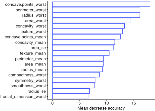
MeanDecreaseAccuracy shows that the contribution of the features. For exmple, removing concave.points_worst would decrease the accuracy by 18.0%. The higher the MeanDecreaseAccuracy of the features, the more they contribute to the model.
Cross validation
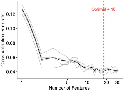
5 replicates for the 5-folds cross-validation to obtain the mean error in order to avoid the over-fitting and under-fitting. Meanwhile, the optimal number of features is selected according to the number with the mean error.
error.cv <- c()
for (i in 1:5){
  print(i)
  set.seed(i)
  fit <- rfcv(trainx = X_train,
              trainy = y_train,
              cv.fold = 5,
              scale = "log",
              step = 0.9)
  error.cv <- cbind(error.cv, fit$error.cv)
}

n.var <- as.numeric(rownames(error.cv))
colnames(error.cv) <- paste('error', 1:5, sep = '.')
err.mean <- apply(error.cv, 1, mean)
err.df <- data.frame(num = n.var,
                     err.mean = err.mean,
                     error.cv)
head(err.df[, 1:6])
   num   err.mean    error.1    error.2    error.3    error.4
30  30 0.04110276 0.03759398 0.04260652 0.04260652 0.04260652
27  27 0.04160401 0.04010025 0.04010025 0.04761905 0.04010025
24  24 0.04260652 0.04260652 0.04260652 0.04260652 0.04761905
22  22 0.04360902 0.04260652 0.04260652 0.04511278 0.04511278
20  20 0.04210526 0.04260652 0.04511278 0.04260652 0.04260652
18  18 0.04060150 0.04260652 0.04260652 0.04010025 0.04260652
- optimal number of biomarkers chosen by min cv.error
optimal <- err.df$num[which(err.df$err.mean == min(err.df$err.mean))]
main_theme <-
  theme(
    panel.background = element_blank(),
    panel.grid = element_blank(),
    axis.line.x = element_line(linewidth = 0.5, color = "black"),
    axis.line.y = element_line(linewidth = 0.5, color = "black"),
    axis.ticks = element_line(color = "black"),
    axis.text = element_text(color = "black", size = 12),
    legend.position = "right",
    legend.background = element_blank(),
    legend.key = element_blank(),
    legend.text = element_text(size = 12),
    text = element_text(family = "sans", size = 12))

pl <-
  ggplot(data = err.df, aes(x = err.df$num)) +
    geom_line(aes(y = err.df$error.1), color = 'grey', size = 0.5) +
    geom_line(aes(y = err.df$error.2), color = 'grey', size = 0.5) +
    geom_line(aes(y = err.df$error.3), color = 'grey', size = 0.5) +
    geom_line(aes(y = err.df$error.4), color = 'grey', size = 0.5) +
    geom_line(aes(y = err.df$error.5), color = 'grey', size = 0.5) +
    geom_line(aes(y = err.df$err.mean), color = 'black', size = 0.5) +
    geom_vline(xintercept = optimal, color = 'red', lwd = 0.36, linetype = 2) +
    coord_trans(x = "log2") +
    scale_x_continuous(breaks = c(1, 5, 10, 20, 30)) +
    labs(x = 'Number of Species ', y = 'Cross-validation error rate') +
    annotate("text",
             x = optimal,
             y = max(err.df$err.mean),
             label = paste("Optimal = ", optimal, sep = ""),
             color = "red") +
    main_theme
pl
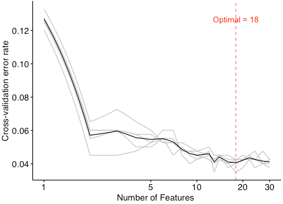
Since the figure shows that the model had a minimum error rate when the number of features was 18, the optimal number of biomarkers is 18.
- importance of optimal biomarker
Displaying the MeanDecreaseAccuracy of the best biomarkers
imp_biomarker[1:optimal, ] %>%
  dplyr::select(Features, MeanDecreaseAccuracy) %>%
  dplyr::arrange(MeanDecreaseAccuracy) %>%
  dplyr::mutate(Features = forcats::fct_inorder(Features)) %>%
  ggplot(aes(x = Features, y = MeanDecreaseAccuracy))+
    geom_bar(stat = "identity", fill = "white", color = "blue") +
    labs(x = "", y = "Mean decrease accuracy") +
    coord_flip() +
    main_theme
Rebuilding model by the optimal biomarkers
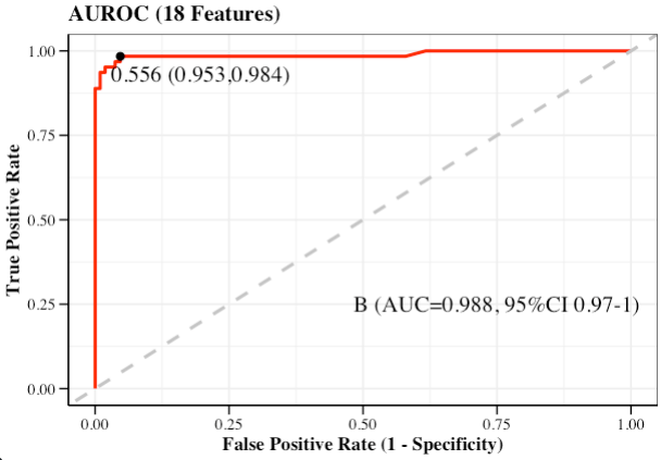
Here, we used the new candidates to rebuild the RF model, and the accuracy of the new model increased by 0.5% (the OOB error rate decreased from 4.26% to 3.76%).
selected_columns <- c("Group", imp_biomarker[1:optimal, ]$Features)

trainData_optimal <- trainData %>%
  dplyr::select(all_of(selected_columns))

testData_optimal <- testData %>%
  dplyr::select(all_of(selected_columns))

set.seed(123)
rf_fit_optimal <- randomForest(Group ~ ., data = trainData_optimal, importance = TRUE, proximity = TRUE)
rf_fit_optimal
Call:
 randomForest(formula = Group ~ ., data = trainData_optimal, importance = TRUE,      proximity = TRUE)
               Type of random forest: classification
                     Number of trees: 500
No. of variables tried at each split: 4

        OOB estimate of  error rate: 3.76%
Confusion matrix:
    B   M class.error
B 242   8  0.03200000
M   7 142  0.04697987
- ConfusionMatrix
group_names <- c("B", "M")
pred_raw <- predict(rf_fit_optimal, newdata = testData_optimal, type = "response")
print(caret::confusionMatrix(pred_raw, testData_optimal$Group))
pred_prob <- predict(rf_fit_optimal, newdata = testData_optimal, type = "prob")
Confusion Matrix and Statistics

          Reference
Prediction   B   M
         B 105   3
         M   2  60

               Accuracy : 0.9706
                 95% CI : (0.9327, 0.9904)
    No Information Rate : 0.6294
    P-Value [Acc > NIR] : <2e-16

                  Kappa : 0.9367

 Mcnemar's Test P-Value : 1

            Sensitivity : 0.9813
            Specificity : 0.9524
         Pos Pred Value : 0.9722
         Neg Pred Value : 0.9677
             Prevalence : 0.6294
         Detection Rate : 0.6176
   Detection Prevalence : 0.6353
      Balanced Accuracy : 0.9668

       'Positive' Class : B
- performance of classifier
Evaluate_index <- function(
    DataTest,
    PredProb = pred_prob,
    label = group_names[1],
    PredRaw = pred_raw) {

  # DataTest = testData
  # PredProb = pred_prob
  # label = group_names[1]
  # PredRaw = pred_raw

  # ROC object
  rocobj <- roc(DataTest$Group, PredProb[, 1])

  # confusionMatrix
  con_matrix <- table(PredRaw, DataTest$Group)

  # index
  TP <- con_matrix[1, 1]
  FN <- con_matrix[2, 1]
  FP <- con_matrix[1, 2]
  TN <- con_matrix[2, 2]

  rocbj_df <- data.frame(threshold = round(rocobj$thresholds, 3),
                         sensitivities = round(rocobj$sensitivities, 3),
                         specificities = round(rocobj$specificities, 3),
                         value = rocobj$sensitivities +
                           rocobj$specificities)
  max_value_row <- which(max(rocbj_df$value) == rocbj_df$value)[1]

  threshold <- rocbj_df$threshold[max_value_row]
  sen <- round(TP / (TP + FN), 3) # caret::sensitivity(con_matrix)
  spe <- round(TN / (TN + FP), 3) # caret::specificity(con_matrix)
  acc <- round((TP + TN) / (TP + TN + FP + FN), 3) # Accuracy
  pre <- round(TP / (TP + FP), 3) # precision
  rec <- round(TP / (TP + FN), 3) # recall
  #F1S <- round(2 * TP / (TP + TN + FP + FN + TP - TN), 3)# F1-Score
  F1S <- round(2 * TP / (2 * TP + FP + FN), 3)# F1-Score
  youden <- sen + spe - 1 # youden index

  index_df <- data.frame(Index = c("Threshold", "Sensitivity",
                                   "Specificity", "Accuracy",
                                   "Precision", "Recall",
                                   "F1 Score", "Youden index"),
                         Value = c(threshold, sen, spe,
                                   acc, pre, rec, F1S, youden)) %>%
    stats::setNames(c("Index", label))

  return(index_df)
}

Evaluate_index(
    DataTest = testData,
    PredProb = pred_prob,
    label = group_names[1],
    PredRaw = pred_raw)
         Index     B
1    Threshold 0.556
2  Sensitivity 0.981
3  Specificity 0.952
4     Accuracy 0.971
5    Precision 0.972
6       Recall 0.981
7     F1 Score 0.977
8 Youden index 0.933
- AUROC
AUROC <- function(
    DataTest,
    PredProb = pred_prob,
    label = group_names[1],
    DataProf = profile) {

  # ROC object
  rocobj <- roc(DataTest$Group, PredProb[, 1])

  # Youden index: cutoff point
  # plot(rocobj,
  #      legacy.axes = TRUE,
  #      of = "thresholds",
  #      thresholds = "best",
  #      print.thres="best")

  # AUROC data
  roc <- data.frame(tpr = rocobj$sensitivities,
                    fpr = 1 - rocobj$specificities)

  # AUC 95% CI
  rocobj_CI <- roc(DataTest$Group, PredProb[, 1],
                   ci = TRUE, percent = TRUE)
  roc_CI <- round(as.numeric(rocobj_CI$ci)/100, 3)
  roc_CI_lab <- paste0(label,
                       " (", "AUC=", roc_CI[2],
                       ", 95%CI ", roc_CI[1], "-", roc_CI[3],
                       ")")
  # ROC dataframe
  rocbj_df <- data.frame(threshold = round(rocobj$thresholds, 3),
                         sensitivities = round(rocobj$sensitivities, 3),
                         specificities = round(rocobj$specificities, 3),
                         value = rocobj$sensitivities +
                           rocobj$specificities)
  max_value_row <- which(max(rocbj_df$value) == rocbj_df$value)
  threshold <- rocbj_df$threshold[max_value_row]

  # plot
  pl <- ggplot(data = roc, aes(x = fpr, y = tpr)) +
    geom_path(color = "red", size = 1) +
    geom_abline(intercept = 0, slope = 1,
                color = "grey", size = 1, linetype = 2) +
    labs(x = "False Positive Rate (1 - Specificity)",
         y = "True Positive Rate",
         title = paste0("AUROC (", DataProf, " Features)")) +
    annotate("text",
             x = 1 - rocbj_df$specificities[max_value_row] + 0.15,
             y = rocbj_df$sensitivities[max_value_row] - 0.05,
             label = paste0(threshold, " (",
                            rocbj_df$specificities[max_value_row], ",",
                            rocbj_df$sensitivities[max_value_row], ")"),
             size=5, family="serif") +
    annotate("point",
             x = 1 - rocbj_df$specificities[max_value_row],
             y = rocbj_df$sensitivities[max_value_row],
             color = "black", size = 2) +
    annotate("text",
             x = .75, y = .25,
             label = roc_CI_lab,
             size = 5, family = "serif") +
    coord_cartesian(xlim = c(0, 1), ylim = c(0, 1)) +
    theme_bw() +
    theme(panel.background = element_rect(fill = "transparent"),
          plot.title = element_text(color = "black", size = 14, face = "bold"),
          axis.ticks.length = unit(0.4, "lines"),
          axis.ticks = element_line(color = "black"),
          axis.line = element_line(size = .5, color = "black"),
          axis.title = element_text(color = "black", size = 12, face = "bold"),
          axis.text = element_text(color = "black", size = 10),
          text = element_text(size = 8, color = "black", family = "serif"))

  res <- list(rocobj = rocobj,
              roc_CI = roc_CI_lab,
              roc_pl = pl)

  return(res)
}

AUROC_res <- AUROC(
    DataTest = testData,
    PredProb = pred_prob,
    label = group_names[1],
    DataProf = optimal)

AUROC_res$roc_pl
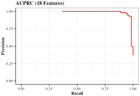
- AUPRC
AUPRC <- function(
    DataTest,
    PredProb = pred_prob,
    DataProf = optimal) {

  # ROC object
  rocobj <- roc(DataTest$Group, PredProb[, 1])

  # p-r value
  dat_PR <- coords(rocobj, "all", ret = c("precision", "recall"))

  # AUPRC data
  prc <- data.frame(precision = dat_PR$precision,
                    recall = dat_PR$recall)

  # plot
  pl <- ggplot(data = prc, aes(x = recall, y = precision)) +
    geom_path(color = "red", size = 1) +
    labs(x = "Recall",
         y = "Precision",
         title = paste0("AUPRC (", DataProf, " Features)")) +
    coord_cartesian(xlim = c(0, 1), ylim = c(0, 1)) +
    theme_bw() +
    theme(panel.background = element_rect(fill = "transparent"),
          plot.title = element_text(color = "black", size = 14, face = "bold"),
          axis.ticks.length = unit(0.4, "lines"),
          axis.ticks = element_line(color = "black"),
          axis.line = element_line(size = .5, color = "black"),
          axis.title = element_text(color = "black", size = 12, face = "bold"),
          axis.text = element_text(color = "black", size = 10),
          text = element_text(size = 8, color = "black", family = "serif"))

  res <- list(dat_PR = dat_PR,
              PC_pl = pl)

  return(res)
}

AUPRC_res <- AUPRC(
    DataTest = testData,
    PredProb = pred_prob,
    DataProf = optimal)

AUPRC_res$PC_pl
systemic information
devtools::session_info()
─ Session info ─────────────────────────────────────────────────────────────────────────────────────────────────────────
 setting  value
 version  R version 4.1.2 (2021-11-01)
 os       macOS Monterey 12.2.1
 system   x86_64, darwin17.0
 ui       RStudio
 language (EN)
 collate  en_US.UTF-8
 ctype    en_US.UTF-8
 tz       Asia/Shanghai
 date     2023-04-27
 rstudio  2022.07.2+576 Spotted Wakerobin (desktop)
 pandoc   2.19.2 @ /Applications/RStudio.app/Contents/MacOS/quarto/bin/tools/ (via rmarkdown)

─ Packages ─────────────────────────────────────────────────────────────────────────────────────────────────────────────
 package      * version    date (UTC) lib source
 assertthat     0.2.1      2019-03-21 [1] CRAN (R 4.1.0)
 blogdown       1.13.3     2022-11-01 [1] Github (rstudio/blogdown@5dddefa)
 brio           1.1.3      2021-11-30 [1] CRAN (R 4.1.0)
 cachem         1.0.6      2021-08-19 [1] CRAN (R 4.1.0)
 callr          3.7.0      2021-04-20 [1] CRAN (R 4.1.0)
 caret        * 6.0-92     2022-04-19 [1] CRAN (R 4.1.2)
 class          7.3-20     2022-01-13 [1] CRAN (R 4.1.2)
 cli            3.4.1      2022-09-23 [1] CRAN (R 4.1.2)
 codetools      0.2-18     2020-11-04 [1] CRAN (R 4.1.2)
 colorspace     2.0-3      2022-02-21 [1] CRAN (R 4.1.2)
 crayon         1.5.0      2022-02-14 [1] CRAN (R 4.1.2)
 data.table   * 1.14.6     2022-11-16 [1] CRAN (R 4.1.2)
 DBI            1.1.2      2021-12-20 [1] CRAN (R 4.1.0)
 desc           1.4.1      2022-03-06 [1] CRAN (R 4.1.2)
 devtools       2.4.3      2021-11-30 [1] CRAN (R 4.1.0)
 digest         0.6.30     2022-10-18 [1] CRAN (R 4.1.2)
 dplyr        * 1.0.10     2022-09-01 [1] CRAN (R 4.1.2)
 e1071          1.7-9      2021-09-16 [1] CRAN (R 4.1.0)
 ellipsis       0.3.2      2021-04-29 [1] CRAN (R 4.1.0)
 evaluate       0.17       2022-10-07 [1] CRAN (R 4.1.2)
 fansi          1.0.2      2022-01-14 [1] CRAN (R 4.1.2)
 farver         2.1.0      2021-02-28 [1] CRAN (R 4.1.0)
 fastmap        1.1.0      2021-01-25 [1] CRAN (R 4.1.0)
 forcats        0.5.1      2021-01-27 [1] CRAN (R 4.1.0)
 foreach        1.5.2      2022-02-02 [1] CRAN (R 4.1.2)
 fs             1.5.2      2021-12-08 [1] CRAN (R 4.1.0)
 future         1.28.0     2022-09-02 [1] CRAN (R 4.1.2)
 future.apply   1.8.1      2021-08-10 [1] CRAN (R 4.1.0)
 generics       0.1.2      2022-01-31 [1] CRAN (R 4.1.2)
 ggplot2      * 3.4.0      2022-11-04 [1] CRAN (R 4.1.2)
 globals        0.16.1     2022-08-28 [1] CRAN (R 4.1.2)
 glue           1.6.2      2022-02-24 [1] CRAN (R 4.1.2)
 gower          1.0.0      2022-02-03 [1] CRAN (R 4.1.2)
 gtable         0.3.0      2019-03-25 [1] CRAN (R 4.1.0)
 hardhat        1.2.0      2022-06-30 [1] CRAN (R 4.1.2)
 htmltools      0.5.3      2022-07-18 [1] CRAN (R 4.1.2)
 ipred          0.9-12     2021-09-15 [1] CRAN (R 4.1.0)
 iterators      1.0.14     2022-02-05 [1] CRAN (R 4.1.2)
 jsonlite       1.8.3      2022-10-21 [1] CRAN (R 4.1.2)
 knitr          1.40       2022-08-24 [1] CRAN (R 4.1.2)
 labeling       0.4.2      2020-10-20 [1] CRAN (R 4.1.0)
 lattice      * 0.20-45    2021-09-22 [1] CRAN (R 4.1.2)
 lava           1.6.10     2021-09-02 [1] CRAN (R 4.1.0)
 lifecycle      1.0.3      2022-10-07 [1] CRAN (R 4.1.2)
 listenv        0.8.0      2019-12-05 [1] CRAN (R 4.1.0)
 lubridate      1.8.0      2021-10-07 [1] CRAN (R 4.1.0)
 magrittr       2.0.3      2022-03-30 [1] CRAN (R 4.1.2)
 MASS           7.3-55     2022-01-13 [1] CRAN (R 4.1.2)
 Matrix         1.4-0      2021-12-08 [1] CRAN (R 4.1.0)
 memoise        2.0.1      2021-11-26 [1] CRAN (R 4.1.0)
 ModelMetrics   1.2.2.2    2020-03-17 [1] CRAN (R 4.1.0)
 munsell        0.5.0      2018-06-12 [1] CRAN (R 4.1.0)
 nlme           3.1-155    2022-01-13 [1] CRAN (R 4.1.2)
 nnet           7.3-17     2022-01-13 [1] CRAN (R 4.1.2)
 parallelly     1.32.1     2022-07-21 [1] CRAN (R 4.1.2)
 pillar         1.7.0      2022-02-01 [1] CRAN (R 4.1.2)
 pkgbuild       1.3.1      2021-12-20 [1] CRAN (R 4.1.0)
 pkgconfig      2.0.3      2019-09-22 [1] CRAN (R 4.1.0)
 pkgload        1.2.4      2021-11-30 [1] CRAN (R 4.1.0)
 plyr           1.8.6      2020-03-03 [1] CRAN (R 4.1.0)
 prettyunits    1.1.1      2020-01-24 [1] CRAN (R 4.1.0)
 pROC         * 1.18.0     2021-09-03 [1] CRAN (R 4.1.0)
 processx       3.5.2      2021-04-30 [1] CRAN (R 4.1.0)
 prodlim        2019.11.13 2019-11-17 [1] CRAN (R 4.1.0)
 proxy          0.4-26     2021-06-07 [1] CRAN (R 4.1.0)
 ps             1.6.0      2021-02-28 [1] CRAN (R 4.1.0)
 purrr          0.3.4      2020-04-17 [1] CRAN (R 4.1.0)
 R6             2.5.1      2021-08-19 [1] CRAN (R 4.1.0)
 randomForest * 4.7-1      2022-02-03 [1] CRAN (R 4.1.2)
 Rcpp           1.0.10     2023-01-22 [1] CRAN (R 4.1.2)
 recipes        1.0.1      2022-07-07 [1] CRAN (R 4.1.2)
 remotes        2.4.2      2021-11-30 [1] CRAN (R 4.1.0)
 reshape2       1.4.4      2020-04-09 [1] CRAN (R 4.1.0)
 rlang          1.0.6      2022-09-24 [1] CRAN (R 4.1.2)
 rmarkdown      2.17       2022-10-07 [1] CRAN (R 4.1.2)
 rpart          4.1.16     2022-01-24 [1] CRAN (R 4.1.2)
 rprojroot      2.0.2      2020-11-15 [1] CRAN (R 4.1.0)
 rstudioapi     0.13       2020-11-12 [1] CRAN (R 4.1.0)
 scales         1.2.1      2022-08-20 [1] CRAN (R 4.1.2)
 sessioninfo    1.2.2      2021-12-06 [1] CRAN (R 4.1.0)
 stringi        1.7.8      2022-07-11 [1] CRAN (R 4.1.2)
 stringr        1.4.1      2022-08-20 [1] CRAN (R 4.1.2)
 survival       3.4-0      2022-08-09 [1] CRAN (R 4.1.2)
 testthat       3.1.2      2022-01-20 [1] CRAN (R 4.1.2)
 tibble       * 3.1.8      2022-07-22 [1] CRAN (R 4.1.2)
 tidyselect     1.1.2      2022-02-21 [1] CRAN (R 4.1.2)
 timeDate       3043.102   2018-02-21 [1] CRAN (R 4.1.0)
 usethis        2.1.5      2021-12-09 [1] CRAN (R 4.1.0)
 utf8           1.2.2      2021-07-24 [1] CRAN (R 4.1.0)
 vctrs          0.5.1      2022-11-16 [1] CRAN (R 4.1.2)
 withr          2.5.0      2022-03-03 [1] CRAN (R 4.1.2)
 xfun           0.34       2022-10-18 [1] CRAN (R 4.1.2)
 yaml           2.3.6      2022-10-18 [1] CRAN (R 4.1.2)

 [1] /Library/Frameworks/R.framework/Versions/4.1/Resources/library
Summary
Random Forest classification with optimal features using R.
- Data partition.
- Features importance.
- Cross validation for OOB errors.
- The optimal features for rebuilding model.
- Performance Evaluation based on optimal features.
- Finalize results with AUROC and AUPRC etc.