Predictive Model using Random Forest
Random Forest, a ensemble machine learning algorithm with multiple decision trees could be used for classification or regression algorithm, and it has an elegant way of dealing with nonlinear or linear data.
Random forest aims to reduce the previously mentioned correlation issue by choosing only a subsample of the feature space at each split. Essentially, it aims to make the trees de-correlated and prune the trees by setting a stopping criteria for node splits, which I will cover in more detail later.
Important Parameters
- number of estimators: the number of trees for constructing forest.
- max depth of each tree: the number of features per decision tree.
- max features per split: it affects the performance of the whole dicision tree.
estimator also termed tree and depth control the complexity of the model, with larger estimators would result in better and high density forest and maximum depth helps fighting with overfitting.
Random Forest doesn't require careful preprocessing such as normalization of data. Standardization is an important requirement for many classification models that should be handled when implementing pre-processing. Some models (like neural networks) can perform poorly if pre-processing isn’t considered, so the describe() function is a good indicator for standardization. Fortunately, random forest does not require any pre-processing.
Loading libraries
%matplotlib inline
import matplotlib.pyplot as plt

import pandas as pd
import numpy as np
import time
import random

from sklearn.preprocessing import LabelEncoder
from sklearn.model_selection import train_test_split
from sklearn.ensemble import RandomForestClassifier
from sklearn.metrics import accuracy_score
from sklearn.metrics import roc_curve, auc
from sklearn.metrics import confusion_matrix
from sklearn.model_selection import cross_val_score
from sklearn.metrics import classification_report
from sklearn.model_selection import GridSearchCV, train_test_split

import seaborn as sns
#plt.style.use('fivethirtyeight')
plt.style.use('fivethirtyeight')
sns.set_style("darkgrid")

plt.rcParams['figure.figsize'] = (8, 4)
Importing data
'''
# raw data
data_df = pd.read_table('./dataset/MergeData.tsv', sep="\t", index_col=0)
data = data_df.reset_index(drop=True)
data.head()

# significant species
data_df = pd.read_table('./dataset/MergeData_clr_signif.tsv', sep="\t", index_col=0)
data = data_df.reset_index(drop=True)
data.head()
'''

# CLR-transformed data
data_df = pd.read_table('./dataset/MergeData_clr.tsv', sep="\t", index_col=0)
data = data_df.reset_index(drop=True)
data.head()
| disease | s__Bacteroides_plebeius | s__Bacteroides_dorei | s__Faecalibacterium_prausnitzii | s__Eubacterium_eligens | s__Bacteroides_ovatus | s__Parabacteroides_distasonis | s__Ruminococcus_gnavus | s__Phascolarctobacterium_faecium | s__Bacteroides_uniformis | ... | s__Bacteroides_finegoldii | s__Haemophilus_sp_HMSC71H05 | s__Clostridium_saccharolyticum | s__Streptococcus_anginosus_group | s__Streptococcus_sp_A12 | s__Klebsiella_pneumoniae | s__Bacteroides_coprocola | s__Ruminococcus_lactaris | s__Turicimonas_muris | s__Proteobacteria_bacterium_CAG_139 | |
|---|---|---|---|---|---|---|---|---|---|---|---|---|---|---|---|---|---|---|---|---|---|
| 0 | healthy | 10.262146 | 8.532694 | 7.729839 | 7.605931 | 7.477464 | 7.267232 | 7.074996 | 6.832596 | 6.738413 | ... | -3.441779 | -3.441779 | -3.441779 | -3.441779 | -3.441779 | -3.441779 | -3.441779 | -3.441779 | -3.441779 | -3.441779 |
| 1 | healthy | 7.609333 | 4.466872 | 6.654823 | 4.236672 | 4.697277 | 3.518645 | 2.603642 | -3.929140 | 5.619399 | ... | -3.929140 | -3.929140 | -3.929140 | -3.929140 | -3.929140 | -3.929140 | -3.929140 | -3.929140 | -3.929140 | -3.929140 |
| 2 | healthy | 8.411267 | 7.884081 | 7.668467 | -3.379905 | 6.577229 | 6.474488 | 6.883446 | -3.379905 | 6.725545 | ... | -3.379905 | -3.379905 | -3.379905 | -3.379905 | -3.379905 | -3.379905 | -3.379905 | -3.379905 | -3.379905 | -3.379905 |
| 3 | healthy | 6.261269 | 6.939669 | 5.819509 | 4.064784 | 4.026179 | 7.227381 | 3.407265 | -3.632294 | 6.170285 | ... | -3.632294 | -3.632294 | -3.632294 | -3.632294 | -3.632294 | -3.632294 | -3.632294 | -3.632294 | -3.632294 | -3.632294 |
| 4 | CRC | -0.026692 | 5.697435 | 3.808831 | 4.253082 | 4.284986 | 5.784833 | 6.384592 | -5.007660 | 5.492187 | ... | 4.187313 | 2.872359 | 2.219946 | 0.713786 | -5.007660 | -5.007660 | -5.007660 | -5.007660 | -5.007660 | -5.007660 |
5 rows × 152 columns
Missing values or Occurrence
the occurrence per features
#data.iloc[:, 1:].apply(lambda x: np.count_nonzero(x)/len(x), axis=0)
print("Here's the dimensions of our data frame:\n", data.shape)
print("Here's the data types of our columns:\n", data.dtypes)
Here's the dimensions of our data frame:
 (504, 152)
Here's the data types of our columns:
 disease                                 object
s__Bacteroides_plebeius                float64
s__Bacteroides_dorei                   float64
s__Faecalibacterium_prausnitzii        float64
s__Eubacterium_eligens                 float64
                                        ...
s__Klebsiella_pneumoniae               float64
s__Bacteroides_coprocola               float64
s__Ruminococcus_lactaris               float64
s__Turicimonas_muris                   float64
s__Proteobacteria_bacterium_CAG_139    float64
Length: 152, dtype: object
data.describe()
| s__Bacteroides_plebeius | s__Bacteroides_dorei | s__Faecalibacterium_prausnitzii | s__Eubacterium_eligens | s__Bacteroides_ovatus | s__Parabacteroides_distasonis | s__Ruminococcus_gnavus | s__Phascolarctobacterium_faecium | s__Bacteroides_uniformis | s__Bifidobacterium_longum | ... | s__Bacteroides_finegoldii | s__Haemophilus_sp_HMSC71H05 | s__Clostridium_saccharolyticum | s__Streptococcus_anginosus_group | s__Streptococcus_sp_A12 | s__Klebsiella_pneumoniae | s__Bacteroides_coprocola | s__Ruminococcus_lactaris | s__Turicimonas_muris | s__Proteobacteria_bacterium_CAG_139 | |
|---|---|---|---|---|---|---|---|---|---|---|---|---|---|---|---|---|---|---|---|---|---|
| count | 504.000000 | 504.000000 | 504.000000 | 504.000000 | 504.000000 | 504.000000 | 504.000000 | 504.000000 | 504.000000 | 504.000000 | ... | 504.000000 | 504.000000 | 504.000000 | 504.000000 | 504.000000 | 504.000000 | 504.000000 | 504.000000 | 504.000000 | 504.000000 |
| mean | 1.256825 | 2.927299 | 5.667281 | 1.616724 | 3.307470 | 4.681808 | 3.345991 | -0.456599 | 6.187024 | 2.897217 | ... | -1.050304 | -2.053572 | -1.841538 | -1.708054 | -2.299261 | -1.441218 | -0.784937 | -1.340681 | -2.291258 | -1.626394 |
| std | 5.247064 | 4.821565 | 2.990958 | 4.504301 | 3.605593 | 3.569784 | 3.994830 | 3.804094 | 2.888385 | 3.702841 | ... | 3.734545 | 2.382407 | 2.704140 | 2.416765 | 1.869589 | 3.354881 | 4.252129 | 3.569669 | 2.030418 | 2.930831 |
| min | -5.286399 | -4.671094 | -3.893930 | -4.943353 | -4.341294 | -4.135735 | -4.746337 | -5.286399 | -3.742171 | -4.520503 | ... | -5.061605 | -4.993406 | -5.286399 | -4.993406 | -5.286399 | -5.007660 | -5.286399 | -5.286399 | -5.286399 | -5.286399 |
| 25% | -3.319519 | -2.510933 | 5.642812 | -2.901603 | 1.786175 | 4.290055 | 0.991982 | -3.455534 | 5.611716 | 0.599582 | ... | -3.503629 | -3.597303 | -3.602112 | -3.403795 | -3.571865 | -3.549059 | -3.582676 | -3.576873 | -3.602045 | -3.556058 |
| 50% | -2.118272 | 4.413118 | 6.563336 | 2.013259 | 4.218514 | 5.628107 | 4.270669 | -2.534482 | 6.872015 | 4.003185 | ... | -2.903888 | -2.991046 | -2.946014 | -2.678076 | -2.966351 | -2.945052 | -2.903888 | -2.943603 | -2.989558 | -2.852131 |
| 75% | 6.963744 | 7.264553 | 7.317980 | 6.046958 | 5.716982 | 6.921791 | 6.315415 | 3.635188 | 7.934838 | 5.439522 | ... | 0.770320 | -1.707308 | -1.562814 | -0.247675 | -1.726005 | -0.103514 | 2.553523 | -1.704935 | -1.874005 | -0.813035 |
| max | 11.092608 | 11.372814 | 10.350223 | 10.790908 | 10.995056 | 10.776272 | 10.795287 | 7.801161 | 10.596756 | 11.050896 | ... | 9.794324 | 7.783317 | 6.769775 | 6.339786 | 5.843264 | 10.786159 | 10.152641 | 9.121991 | 5.404423 | 8.287044 |
8 rows × 151 columns
Class balance
Displaying the counts by values and plot
def print_rate(data_frame, col):
try:
col_vals = data_frame[col].value_counts()
col_vals = col_vals.reset_index()
if len(col_vals['index']) > 20:
print('Warning: values in column are more than 20 \nPlease try a column with lower value counts!')
else:
f = lambda x, y: 100 * (x / sum(y))
for i in range(0, len(col_vals['index'])):
print('{0} accounts for {1:.2f}% of the {2} column'\
.format(col_vals['index'][i], f(col_vals[col].iloc[i], col_vals[col]), col))
except KeyError as e:
print('{0}: Not found'.format(e))
print('Please choose the right column name!')
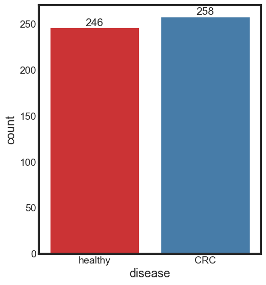
print_rate(data, 'disease')
CRC accounts for 51.19% of the disease column
healthy accounts for 48.81% of the disease column
sns.set_style("white")
sns.set_context({"figure.figsize": (5, 6)})
ax = sns.countplot(x = 'disease', data = data, label = "Count", palette = "Set1")
ax.bar_label(ax.containers[0], fontsize=15)
[Text(0, 0, '246'), Text(0, 0, '258')]
Distribution of features
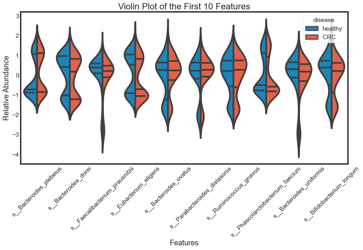
Taking a look at the distribution of each feature and see how they are different between ‘healthy’ and ‘CRC’. To see the distribution of multiple variables, using violin plot, swarm plot or box plot.
Here, we choose 10 features to visualization
- standardizing data and gathering data into long data
from sklearn.preprocessing import StandardScaler


df_features = data.iloc[:, 1:]

scaler = StandardScaler()
scaler.fit(df_features)

features_scaled = scaler.transform(df_features)
features_scaled = pd.DataFrame(data=features_scaled,
                               columns=df_features.columns)

data_scaled = pd.concat([features_scaled, data['disease']], axis=1)

data_scaled_melt = pd.melt(data_scaled, id_vars='disease', var_name='features', value_name='value')
data_scaled_melt.head(10)
| disease | features | value | |
|---|---|---|---|
| 0 | healthy | s__Bacteroides_plebeius | 1.717964 |
| 1 | healthy | s__Bacteroides_plebeius | 1.211882 |
| 2 | healthy | s__Bacteroides_plebeius | 1.364868 |
| 3 | healthy | s__Bacteroides_plebeius | 0.954709 |
| 4 | CRC | s__Bacteroides_plebeius | -0.244859 |
| 5 | CRC | s__Bacteroides_plebeius | -0.364734 |
| 6 | CRC | s__Bacteroides_plebeius | 0.002748 |
| 7 | CRC | s__Bacteroides_plebeius | 1.222586 |
| 8 | CRC | s__Bacteroides_plebeius | 0.547317 |
| 9 | CRC | s__Bacteroides_plebeius | -1.182821 |
- violin plot
def violin_plot(features, name):
    """
    This function creates violin plots of features given in the argument.
    """
    # Create query
    query = ''
    for x in features:
        query += "features == '" + str(x) + "' or "
    query = query[0: -4]

    # Create data for visualization
    plotdata = data_scaled_melt.query(query)

    # Plot figure
    plt.figure(figsize=(12, 6))
    sns.violinplot(x='features',
                   y='value',
                   hue='disease',
                   data=plotdata,
                   split=True,
                   inner="quart")
    plt.xticks(rotation=45)
    plt.title(name)
    plt.xlabel("Features")
    plt.ylabel("Relative Abundance")


violin_plot(data.columns[1:11], "Violin Plot of the First 10 Features")
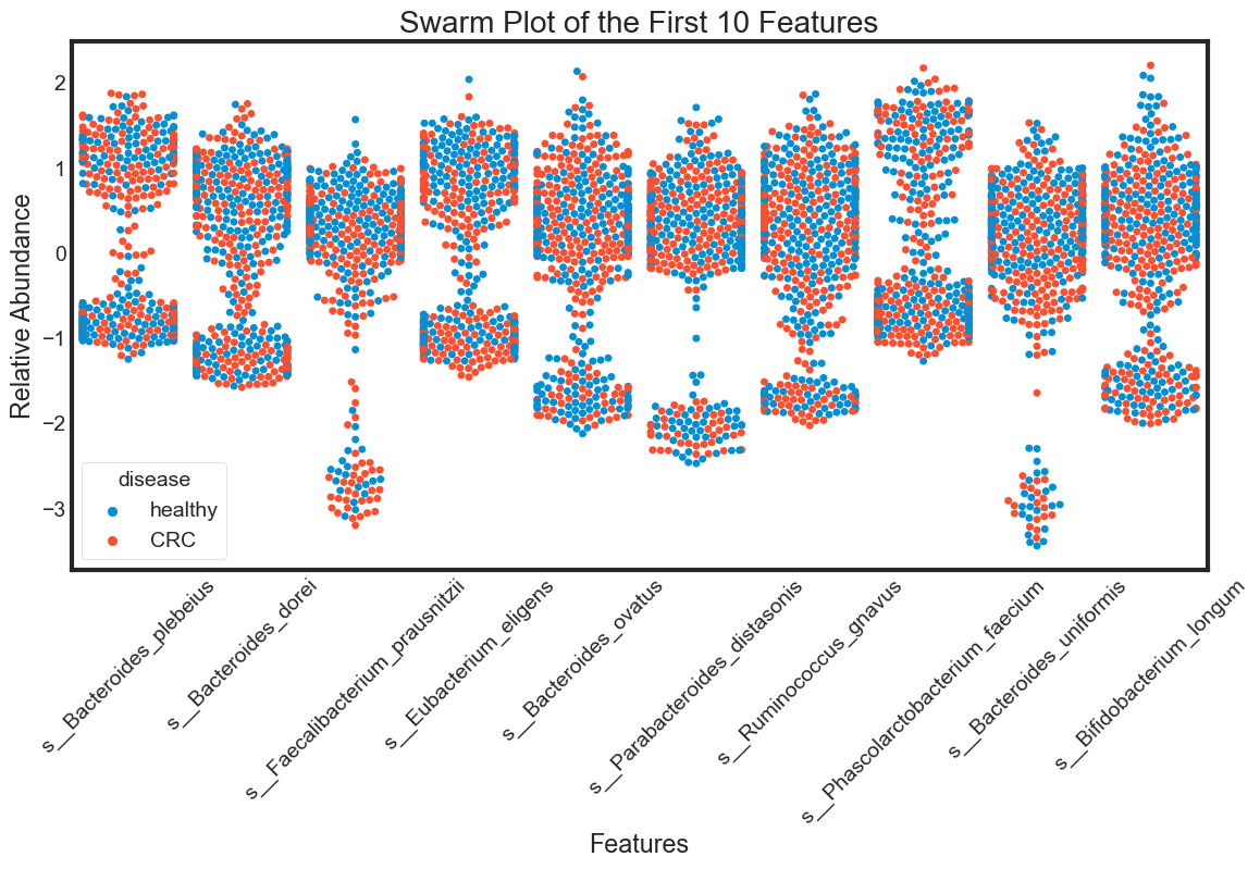
- swarm plot
%%capture --no-display

def swarm_plot(features, name):
    """
    This function creates swarm plots of features given in the argument.
    """
    # Create query
    query = ''
    for x in features:
        query += "features == '" + str(x) + "' or "
    query = query[0:-4]

    # Create data for visualization
    data = data_scaled_melt.query(query)

    # Plot figure
    plt.figure(figsize=(12, 6))
    sns.swarmplot(x='features',
                  y='value',
                  hue='disease',
                  data=data)
    plt.xticks(rotation=45)
    plt.title(name)
    plt.xlabel("Features")
    plt.ylabel("Relative Abundance")

swarm_plot(data.columns[1:11], "Swarm Plot of the First 10 Features")
- boxplot
def box_plot(features, name):
    """
    This function creates box plots of features given in the argument.
    """
    # Create query
    query = ''
    for x in features:
        query += "features == '" + str(x) + "' or "
    query = query[0:-4]

    # Create data for visualization
    data = data_scaled_melt.query(query)

    # Plot figure
    plt.figure(figsize=(12, 6))
    sns.boxplot(x='features',
                y='value',
                hue='disease',
                data=data)
    plt.xticks(rotation=45)
    plt.title(name)
    plt.xlabel("Features")
    plt.ylabel("Relative Abundance")

box_plot(data.columns[1:11], "Box Plot of the First 10 Features")
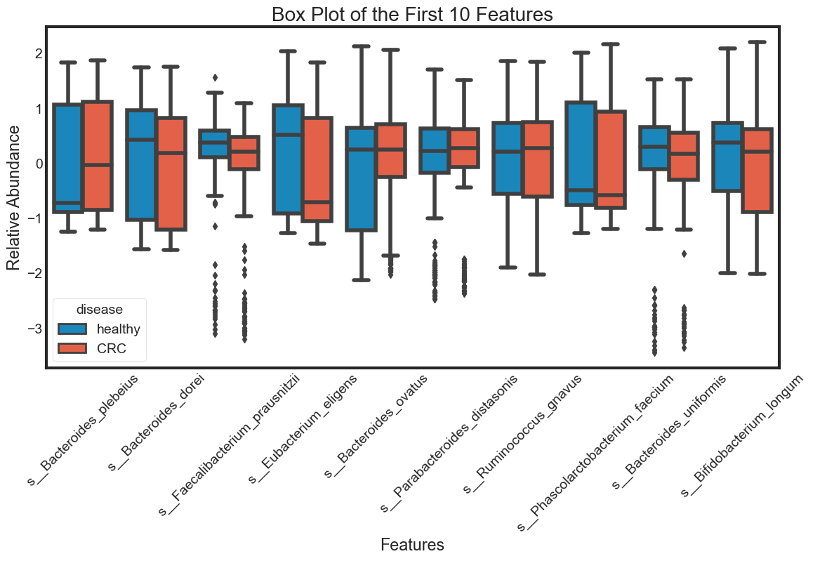
The violin plot is very efficient in comparing distributions of different variables. The classification becomes clear in the swarm plot. Finally, the box plots are useful in comparing median and detecing outliers.
From above plots we can draw some insights from the data:
The median of some features are very different between ‘healthy’ and ‘CRC’. This seperation can be seen clearly in the box plots. They can be very good features for classification. For examples: s__Faecalibacterium_prausnitzii.
However, there are distributions looking similar between ‘healthy’ and ‘CRC’. For examples: s__Bacteroides_plebeius. These features are weak in classifying data.
Some features have similar distributions, thus might be highly correlated with each other. We should not include all these hightly correlated varibles in our predicting model.
Correlation
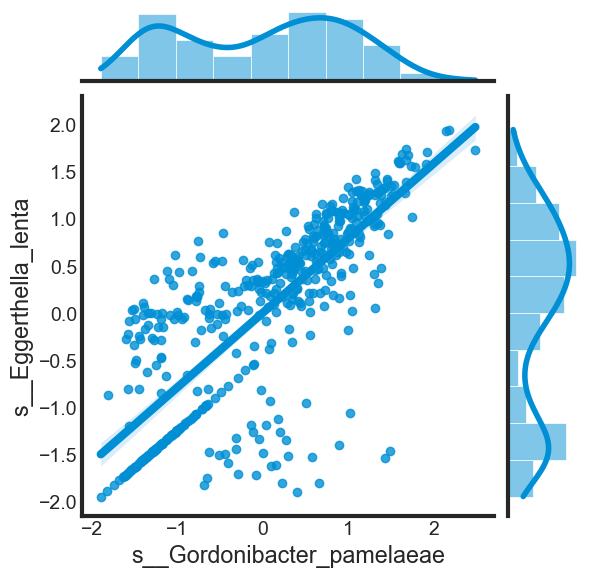
As discussed above, some dependent variables in the dataset might be highly correlated with each other. Let’s explore the correlation of three examples above.
def correlation(data_frame, var):
    """
    1. Print correlation
    2. Create jointplot
    """
    # Print correlation
    print("Correlation: ", data_frame[[var[0], var[1]]].corr().iloc[1, 0])

    # Create jointplot
    plt.figure(figsize=(6, 6))
    sns.jointplot(data = data_frame,
                  x = var[0],
                  y = var[1],
                  kind='reg')
%%capture --no-display
correlation(data_scaled, ['s__Gordonibacter_pamelaeae', 's__Eggerthella_lenta'])
<Figure size 600x600 with 0 Axes>
%%capture --no-display

# Create correlation matrix
corr_mat = data_scaled.iloc[:, 1:100].corr()

# Create mask
mask = np.zeros_like(corr_mat, dtype=np.bool)
mask[np.triu_indices_from(mask, k=1)] = True

# Plot heatmap
plt.figure(figsize=(15, 10))
sns.heatmap(corr_mat,
            annot=True,
            fmt='.1f',
            cmap='RdBu_r',
            vmin=-1,
            vmax=1,
            mask=mask)
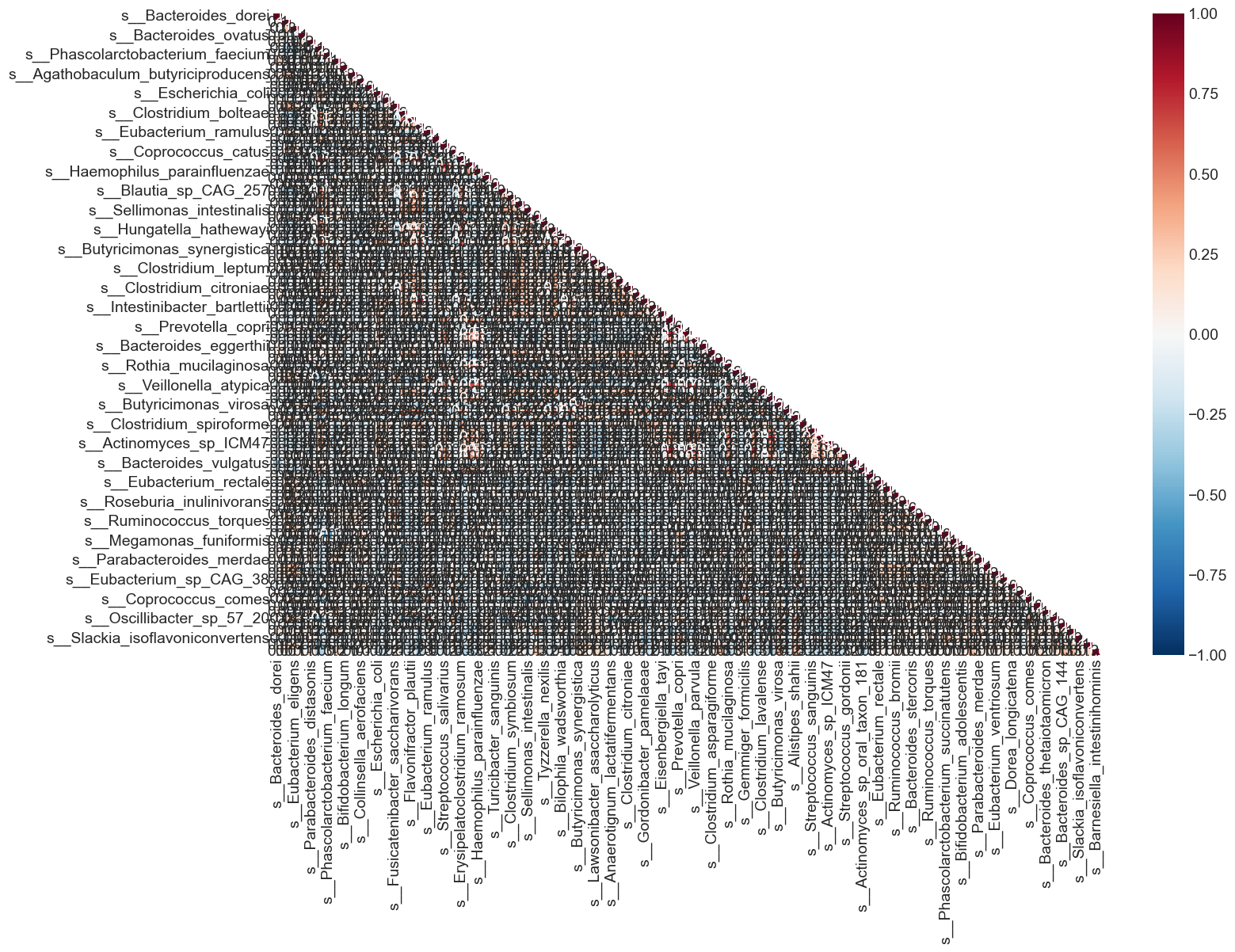
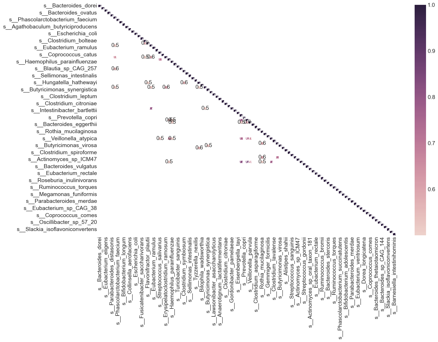
From the heat map, we can see that many variables in the dataset are highly correlated. What are variables having correlation greater than 0.5?
plt.figure(figsize=(15, 10))
sns.heatmap(corr_mat[corr_mat > 0.5],
            annot=True,
            fmt='.1f',
            cmap=sns.cubehelix_palette(200),
            mask=mask)
Feature Selection
Using Univariate Feature Selection (sklearn.feature_selection.SelectKBest) to choose N features with the k highest scores.
from sklearn.feature_selection import SelectKBest, f_classif

df_features = data.iloc[:, 1:]
df_disease = data['disease']

feature_selection = SelectKBest(f_classif, k=100).fit(df_features, df_disease)
selected_features = df_features.columns[feature_selection.get_support()]
print("The N selected features are: ", list(selected_features))
The N selected features are: ['s__Bacteroides_plebeius', 's__Bacteroides_dorei', 's__Faecalibacterium_prausnitzii', 's__Eubacterium_eligens', 's__Bacteroides_ovatus', 's__Parabacteroides_distasonis', 's__Phascolarctobacterium_faecium', 's__Bacteroides_uniformis', 's__Bifidobacterium_longum', 's__Collinsella_aerofaciens', 's__Clostridium_sp_CAG_58', 's__Blautia_wexlerae', 's__Fusicatenibacter_saccharivorans', 's__Eggerthella_lenta', 's__Clostridium_bolteae_CAG_59', 's__Streptococcus_salivarius', 's__Coprococcus_catus', 's__Erysipelatoclostridium_ramosum', 's__Haemophilus_parainfluenzae', 's__Holdemania_filiformis', 's__Turicibacter_sanguinis', 's__Clostridium_symbiosum', 's__Ruthenibacterium_lactatiformans', 's__Sellimonas_intestinalis', 's__Bilophila_wadsworthia', 's__Butyricimonas_synergistica', 's__Parabacteroides_goldsteinii', 's__Anaerotignum_lactatifermentans', 's__Anaerotruncus_colihominis', 's__Intestinibacter_bartlettii', 's__Eisenbergiella_tayi', 's__Prevotella_copri', 's__Clostridium_asparagiforme', 's__Alistipes_indistinctus', 's__Rothia_mucilaginosa', 's__Gemmiger_formicilis', 's__Streptococcus_mitis', 's__Butyricimonas_virosa', 's__Clostridium_aldenense', 's__Alistipes_shahii', 's__Clostridium_spiroforme', 's__Streptococcus_infantis', 's__Lachnospira_pectinoschiza', 's__Eubacterium_rectale', 's__Roseburia_intestinalis', 's__Ruminococcus_bromii', 's__Roseburia_inulinivorans', 's__Anaerostipes_hadrus', 's__Ruminococcus_torques', 's__Roseburia_faecis', 's__Phascolarctobacterium_succinatutens', 's__Megamonas_funiformis', 's__Parabacteroides_merdae', 's__Ruminococcus_bicirculans', 's__Eubacterium_ventriosum', 's__Eubacterium_sp_CAG_38', 's__Dorea_longicatena', 's__Eubacterium_sp_CAG_274', 's__Coprococcus_comes', 's__Bacteroides_caccae', 's__Bacteroides_sp_CAG_144', 's__Odoribacter_splanchnicus', 's__Slackia_isoflavoniconvertens', 's__Bifidobacterium_pseudocatenulatum', 's__Megamonas_hypermegale', 's__Bacteroides_xylanisolvens', 's__Roseburia_hominis', 's__Asaccharobacter_celatus', 's__Adlercreutzia_equolifaciens', 's__Bacteroides_cellulosilyticus', 's__Coprobacter_fastidiosus', 's__Streptococcus_australis', 's__Akkermansia_muciniphila', 's__Streptococcus_thermophilus', 's__Parasutterella_excrementihominis', 's__Allisonella_histaminiformans', 's__Mogibacterium_diversum', 's__Streptococcus_oralis', 's__Eubacterium_sulci', 's__Gemella_sanguinis', 's__Actinomyces_odontolyticus', 's__Gemella_haemolysans', 's__Megasphaera_micronuciformis', 's__Actinomyces_sp_HMSC035G02', 's__Clostridium_clostridioforme', 's__Klebsiella_variicola', 's__Parvimonas_micra', 's__Holdemanella_biformis', 's__Paraprevotella_xylaniphila', 's__Streptococcus_vestibularis', 's__Fusobacterium_mortiferum', 's__Bifidobacterium_dentium', 's__Bacteroides_finegoldii', 's__Clostridium_saccharolyticum', 's__Streptococcus_anginosus_group', 's__Streptococcus_sp_A12', 's__Bacteroides_coprocola', 's__Ruminococcus_lactaris', 's__Turicimonas_muris', 's__Proteobacteria_bacterium_CAG_139']
data_selected = pd.DataFrame(feature_selection.transform(df_features),
                 columns=selected_features)
data_selected.head()
| s__Bacteroides_plebeius | s__Bacteroides_dorei | s__Faecalibacterium_prausnitzii | s__Eubacterium_eligens | s__Bacteroides_ovatus | s__Parabacteroides_distasonis | s__Phascolarctobacterium_faecium | s__Bacteroides_uniformis | s__Bifidobacterium_longum | s__Collinsella_aerofaciens | ... | s__Fusobacterium_mortiferum | s__Bifidobacterium_dentium | s__Bacteroides_finegoldii | s__Clostridium_saccharolyticum | s__Streptococcus_anginosus_group | s__Streptococcus_sp_A12 | s__Bacteroides_coprocola | s__Ruminococcus_lactaris | s__Turicimonas_muris | s__Proteobacteria_bacterium_CAG_139 | |
|---|---|---|---|---|---|---|---|---|---|---|---|---|---|---|---|---|---|---|---|---|---|
| 0 | 10.262146 | 8.532694 | 7.729839 | 7.605931 | 7.477464 | 7.267232 | 6.832596 | 6.738413 | 6.717971 | 6.576766 | ... | -3.441779 | -3.441779 | -3.441779 | -3.441779 | -3.441779 | -3.441779 | -3.441779 | -3.441779 | -3.441779 | -3.441779 |
| 1 | 7.609333 | 4.466872 | 6.654823 | 4.236672 | 4.697277 | 3.518645 | -3.929140 | 5.619399 | 4.429797 | 4.532923 | ... | -3.929140 | -3.929140 | -3.929140 | -3.929140 | -3.929140 | -3.929140 | -3.929140 | -3.929140 | -3.929140 | -3.929140 |
| 2 | 8.411267 | 7.884081 | 7.668467 | -3.379905 | 6.577229 | 6.474488 | -3.379905 | 6.725545 | -3.379905 | -3.379905 | ... | -3.379905 | -3.379905 | -3.379905 | -3.379905 | -3.379905 | -3.379905 | -3.379905 | -3.379905 | -3.379905 | -3.379905 |
| 3 | 6.261269 | 6.939669 | 5.819509 | 4.064784 | 4.026179 | 7.227381 | -3.632294 | 6.170285 | 3.089479 | 5.897842 | ... | 3.295942 | 1.107104 | -3.632294 | -3.632294 | -3.632294 | -3.632294 | -3.632294 | -3.632294 | -3.632294 | -3.632294 |
| 4 | -0.026692 | 5.697435 | 3.808831 | 4.253082 | 4.284986 | 5.784833 | -5.007660 | 5.492187 | 3.893588 | 4.759592 | ... | -5.007660 | -5.007660 | 4.187313 | 2.219946 | 0.713786 | -5.007660 | -5.007660 | -5.007660 | -5.007660 | -5.007660 |
5 rows × 100 columns
Removing variables with high colinearity
def correlation(dataset, threshold):
    col_corr = set() # Set of all the names of deleted columns
    corr_matrix = dataset.corr()
    for i in range(len(corr_matrix.columns)):
        for j in range(i):
            if (corr_matrix.iloc[i, j] >= threshold) and (corr_matrix.columns[j] not in col_corr):
                colname = corr_matrix.columns[i] # getting the name of column
                col_corr.add(colname)
                if colname in dataset.columns:
                    del dataset[colname] # deleting the column from the dataset

correlation(data_selected, 0.6)

data_selected.shape
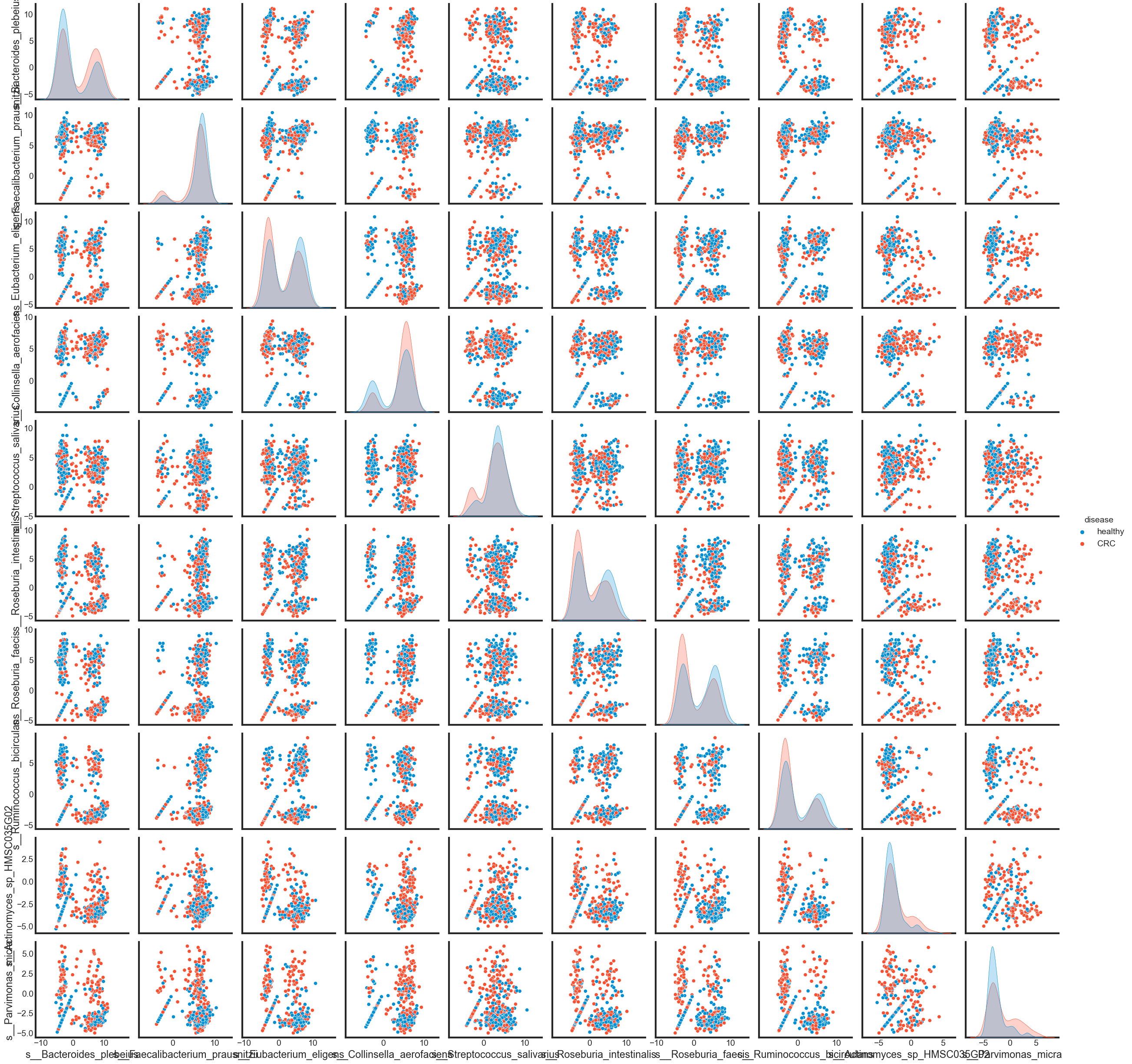
To see how different these features are in ‘CRC’ and in ‘healthy’ by pairplot.
sns.pairplot(pd.concat([data_selected, data['disease']], axis=1), hue='disease')
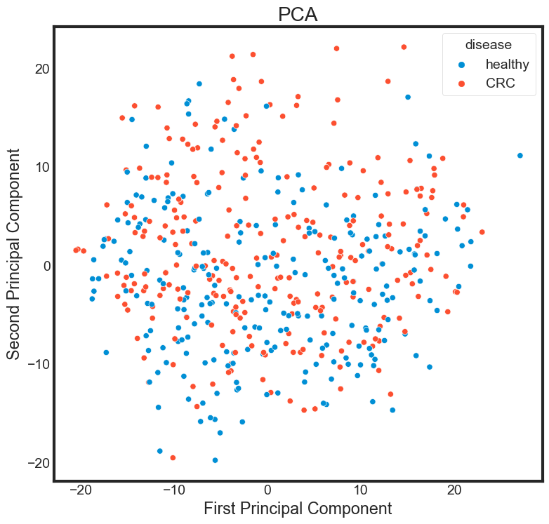
Principal component analysis
from sklearn.decomposition import PCA

pca = PCA(n_components=2)
pca.fit(data_selected)
data_selected_pca = pca.transform(data_selected)

PCA_df = pd.DataFrame()
PCA_df['PCA_1'] = data_selected_pca[:, 0]
PCA_df['PCA_2'] = data_selected_pca[:, 1]


plt.figure(figsize=(8, 8))
sns.scatterplot(data = PCA_df,
                x = 'PCA_1',
                y = 'PCA_2',
                hue=data['disease'])
plt.title("PCA")
plt.xlabel("First Principal Component")
plt.ylabel("Second Principal Component")
Transforming the string label into numeric lable
The RandomForestClassifier in sklearn does not accept string labels for categorical variables.
- 0 = Healthy = Healthy Control
- 1 = CRC = Colorectal Cancer
data['disease'] = data['disease'].map({'healthy':0, 'CRC':1})
data.head(n=6)
| disease | s__Bacteroides_plebeius | s__Bacteroides_dorei | s__Faecalibacterium_prausnitzii | s__Eubacterium_eligens | s__Bacteroides_ovatus | s__Parabacteroides_distasonis | s__Ruminococcus_gnavus | s__Phascolarctobacterium_faecium | s__Bacteroides_uniformis | ... | s__Bacteroides_finegoldii | s__Haemophilus_sp_HMSC71H05 | s__Clostridium_saccharolyticum | s__Streptococcus_anginosus_group | s__Streptococcus_sp_A12 | s__Klebsiella_pneumoniae | s__Bacteroides_coprocola | s__Ruminococcus_lactaris | s__Turicimonas_muris | s__Proteobacteria_bacterium_CAG_139 | |
|---|---|---|---|---|---|---|---|---|---|---|---|---|---|---|---|---|---|---|---|---|---|
| 0 | 0 | 10.262146 | 8.532694 | 7.729839 | 7.605931 | 7.477464 | 7.267232 | 7.074996 | 6.832596 | 6.738413 | ... | -3.441779 | -3.441779 | -3.441779 | -3.441779 | -3.441779 | -3.441779 | -3.441779 | -3.441779 | -3.441779 | -3.441779 |
| 1 | 0 | 7.609333 | 4.466872 | 6.654823 | 4.236672 | 4.697277 | 3.518645 | 2.603642 | -3.929140 | 5.619399 | ... | -3.929140 | -3.929140 | -3.929140 | -3.929140 | -3.929140 | -3.929140 | -3.929140 | -3.929140 | -3.929140 | -3.929140 |
| 2 | 0 | 8.411267 | 7.884081 | 7.668467 | -3.379905 | 6.577229 | 6.474488 | 6.883446 | -3.379905 | 6.725545 | ... | -3.379905 | -3.379905 | -3.379905 | -3.379905 | -3.379905 | -3.379905 | -3.379905 | -3.379905 | -3.379905 | -3.379905 |
| 3 | 0 | 6.261269 | 6.939669 | 5.819509 | 4.064784 | 4.026179 | 7.227381 | 3.407265 | -3.632294 | 6.170285 | ... | -3.632294 | -3.632294 | -3.632294 | -3.632294 | -3.632294 | -3.632294 | -3.632294 | -3.632294 | -3.632294 | -3.632294 |
| 4 | 1 | -0.026692 | 5.697435 | 3.808831 | 4.253082 | 4.284986 | 5.784833 | 6.384592 | -5.007660 | 5.492187 | ... | 4.187313 | 2.872359 | 2.219946 | 0.713786 | -5.007660 | -5.007660 | -5.007660 | -5.007660 | -5.007660 | -5.007660 |
| 5 | 1 | -0.655056 | -1.760058 | 7.171883 | -1.760058 | 0.737587 | 7.421635 | 7.857269 | 6.762199 | 3.025669 | ... | -1.760058 | -1.760058 | 2.682819 | -1.760058 | -0.364194 | -1.760058 | -1.760058 | -1.760058 | -1.760058 | -1.760058 |
6 rows × 152 columns
Creating Train and Test Sets
X = data_selected
Y = data['disease']

x_train, x_test, y_train, y_test = train_test_split(
    X, Y, test_size = 0.30, random_state = 42)
# Cleaning test sets to avoid future warning messages
y_train = y_train.values.ravel()
y_test = y_test.values.ravel()
Fitting Random Forest
- n_estimators: The number of decision tree
- max_depth: The maximum splits for all trees in the forest.
- bootstrap: An indicator of whether or not we want to use bootstrap samples when building trees.
- max_features: The maximum number of features that will be used in node splitting.
- criterion: This is the metric used to asses the stopping criteria for the decision trees.
#%%capture --no-display

fit_rfc = RandomForestClassifier(random_state=123)

np.random.seed(123)
start = time.time()

# hyperparameters Optimzation
param_grid = {
        'n_estimators': [200, 500],
        'max_features': ['auto', 'sqrt', 'log2', None],
        'bootstrap': [True, False],
        'max_depth': [2, 3, 4, 5, 6],
        'criterion': ['gini', 'entropy', 'log_loss']
}

# tuning parameters
cv_rfc = GridSearchCV(estimator = fit_rfc,
                      param_grid=param_grid,
                      cv=5,
                      n_jobs=3)
cv_rfc.fit(X=x_train, y=y_train)

print('Best Parameters using grid search: \n', cv_rfc.best_params_)

end = time.time()

print('Time taken in grid search: {0: .2f}'.format(end - start))
Best Parameters using grid search:
 {'bootstrap': False, 'criterion': 'gini', 'max_depth': 4, 'max_features': 'auto', 'n_estimators': 200}
Time taken in grid search:  273.51
fit_rfc.set_params(bootstrap = True,
                   criterion = 'gini',
                   max_features = 'auto',
                   max_depth = 4,
                   n_estimators = 200)
RandomForestClassifier(max_depth=4, n_estimators=200, oob_score=True,
                       random_state=123, warm_start=True)
Out of Bag Error Rate
Another useful feature of random forest is the concept of an out-of-bag (OOB) error rate. Because only two-thirds of the data are used to train each tree when building the forest, one-third of unseen data can be used in a way that is advantageous to our accuracy metrics without being as computationally expensive as something like cross validation, for instance.
%%capture --no-display

fit_rfc.set_params(warm_start=True,
                   oob_score=True)

min_estimators = 15
max_estimators = 1000

error_rate = {}

for i in range(min_estimators, max_estimators + 1):
    fit_rfc.set_params(n_estimators = i)
    fit_rfc.fit(x_train, y_train)

    oob_error = 1 - fit_rfc.oob_score_
    error_rate[i] = oob_error

oob_series = pd.Series(error_rate)

fig, ax = plt.subplots(figsize=(10, 10))

ax.set_facecolor('#fafafa')

oob_series.plot(kind='line',
                color = 'red')
plt.axhline(0.4,
            color='#875FDB',
            linestyle='--')
plt.axhline(0.34,
            color='#875FDB',
            linestyle='--')
plt.xlabel('n_estimators')
plt.ylabel('OOB Error Rate')
plt.title('OOB Error Rate Across various Forest sizes \n(From 15 to 1000 trees)')
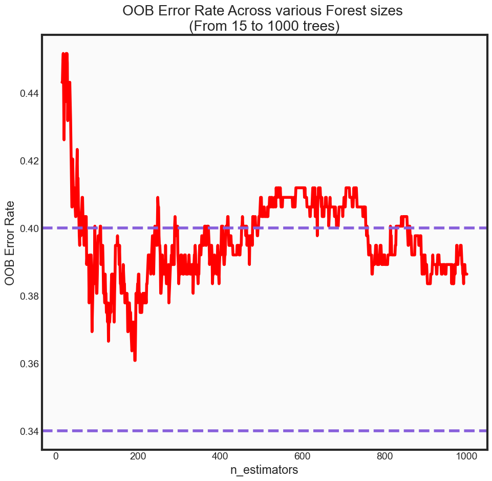
print('OOB Error rate for 200 trees is: {0:.5f}'.format(oob_series[200]))
OOB Error rate for 200 trees is: 0.38352
Building model of optimal parameters
rfc_final = RandomForestClassifier(bootstrap = True,
                                   criterion = 'gini',
                                   max_features = 'auto',
                                   max_depth = 4,
                                   n_estimators = 200,
                                   random_state = 123)
rfc_final.fit(x_train, y_train)

classifier_score = rfc_final.score(x_train, y_train)
print('\nThe classifier accuracy score is {:03.2f}\n'.format(classifier_score))
The classifier accuracy score is 0.95
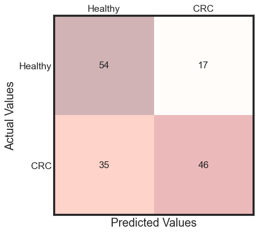
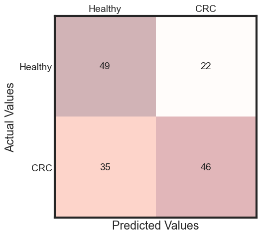
The performance of model on testData
%%capture --no-display

%matplotlib inline
import matplotlib.pyplot as plt
from IPython.display import Image, display
from sklearn import metrics, preprocessing

predicted = rfc_final.predict(x_test)
accuracy = accuracy_score(y_test, predicted)

cm = metrics.confusion_matrix(y_test, predicted)

fig, ax = plt.subplots(figsize=(5, 5))
ax.matshow(cm, cmap=plt.cm.Reds, alpha=0.3)
for i in range(cm.shape[0]):
     for j in range(cm.shape[1]):
         ax.text(x=j, y=i,
                s=cm[i, j],
                va='center', ha='center')
plt.xlabel('Predicted Values', )
plt.ylabel('Actual Values')

ax.set_xticklabels([''] + ['Healthy', "CRC"])
ax.set_yticklabels([''] + ['Healthy', "CRC"])

plt.show()
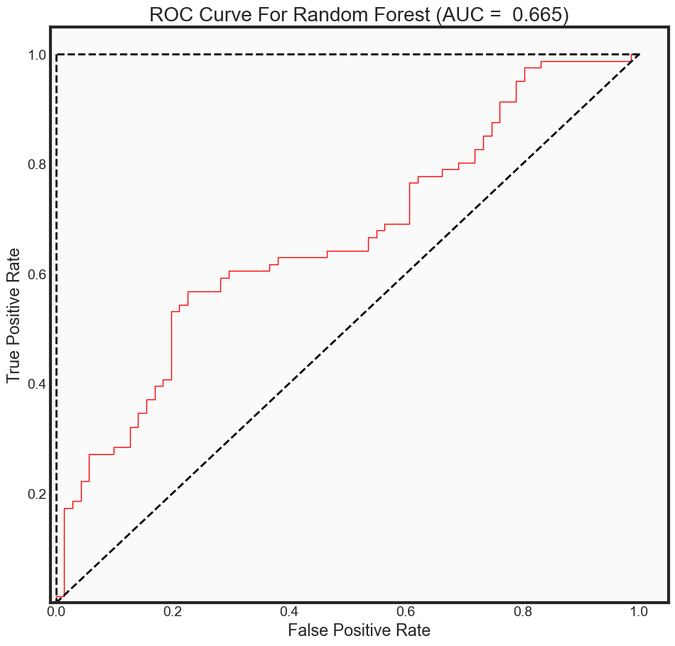
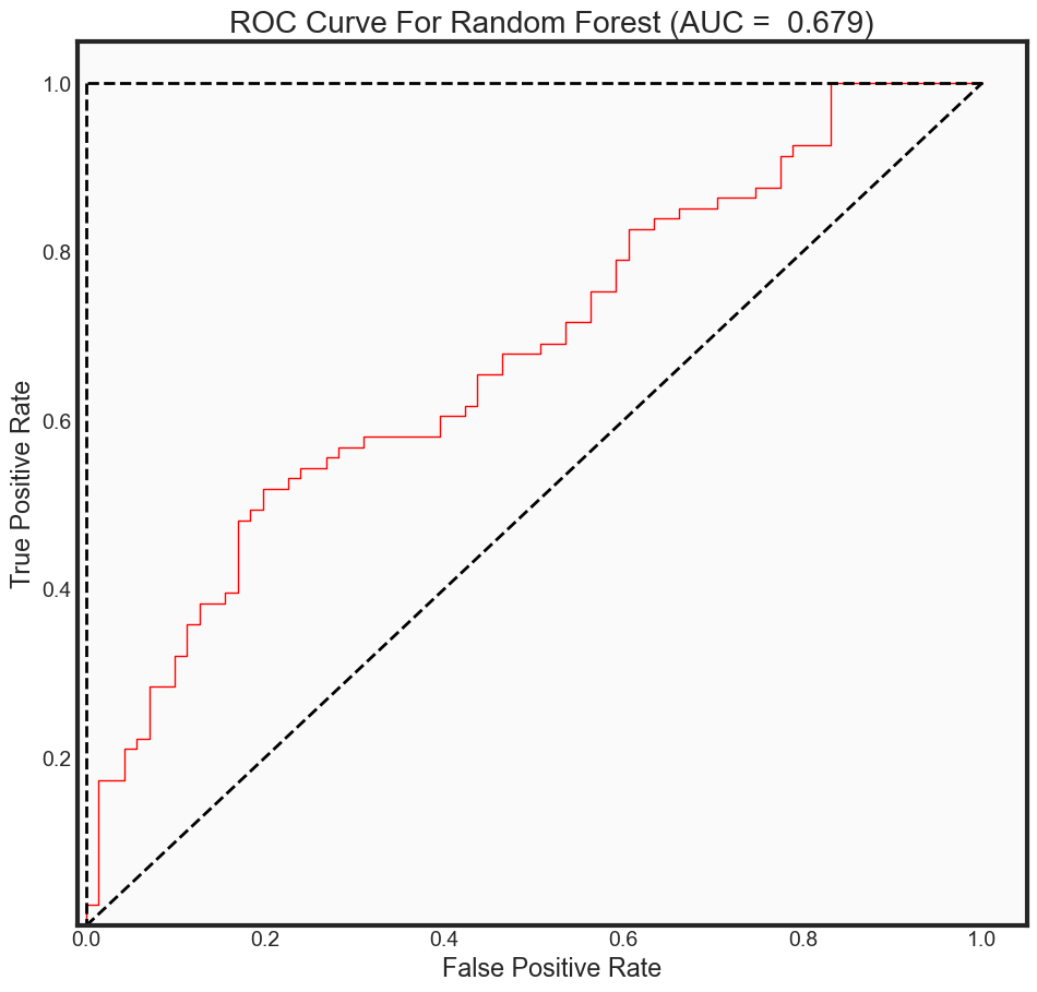
ROC Curve Metrics
# We grab the second array from the output which corresponds to
# to the predicted probabilites of positive classes
# Ordered wrt fit.classes_ in our case [0, 1] where 1 is our positive class
predictions_prob = rfc_final.predict_proba(x_test)[:, 1]

fpr2, tpr2, _ = roc_curve(y_test,
                          predictions_prob,
                          pos_label = 1)

auc_rf = auc(fpr2, tpr2)

print("The AUC for model is: {0: .4f}" .format(auc_rf))
The AUC for model is: 0.6653
def plot_roc_curve(fpr, tpr, auc, estimator, xlim=None, ylim=None):
    """
    Purpose
    ----------
    Function creates ROC Curve for respective model given selected parameters.
    Optional x and y limits to zoom into graph

    Parameters
    ----------
    * fpr: Array returned from sklearn.metrics.roc_curve for increasing
            false positive rates
    * tpr: Array returned from sklearn.metrics.roc_curve for increasing
            true positive rates
    * auc: Float returned from sklearn.metrics.auc (Area under Curve)
    * estimator: String represenation of appropriate model, can only contain the
    following: ['knn', 'rf', 'nn']
    * xlim: Set upper and lower x-limits
    * ylim: Set upper and lower y-limits
    """
    my_estimators = {'knn': ['Kth Nearest Neighbor', 'deeppink'],
              'rf': ['Random Forest', 'red'],
              'nn': ['Neural Network', 'purple']}

    try:
        plot_title = my_estimators[estimator][0]
        color_value = my_estimators[estimator][1]
    except KeyError as e:
        print("'{0}' does not correspond with the appropriate key inside the estimators dictionary. \
\nPlease refer to function to check `my_estimators` dictionary.".format(estimator))
        raise

    fig, ax = plt.subplots(figsize=(10, 10))
    ax.set_facecolor('#fafafa')

    plt.plot(fpr, tpr,
             color=color_value,
             linewidth=1)
    plt.title('ROC Curve For {0} (AUC = {1: 0.3f})'\
              .format(plot_title, auc))

    plt.plot([0, 1], [0, 1], 'k--', lw=2) # Add Diagonal line
    plt.plot([0, 0], [1, 0], 'k--', lw=2, color = 'black')
    plt.plot([1, 0], [1, 1], 'k--', lw=2, color = 'black')
    if xlim is not None:
        plt.xlim(*xlim)
    if ylim is not None:
        plt.ylim(*ylim)
    plt.xlabel('False Positive Rate')
    plt.ylabel('True Positive Rate')
    plt.show()
    plt.close()

plot_roc_curve(fpr2, tpr2, auc_rf, 'rf',
               xlim=(-0.01, 1.05),
               ylim=(0.001, 1.05))
Classification Report
def print_class_report(predictions, alg_name):
    """
    Purpose
    ----------
    Function helps automate the report generated by the
    sklearn package. Useful for multiple model comparison

    Parameters:
    ----------
    predictions: The predictions made by the algorithm used
    alg_name: String containing the name of the algorithm used

    Returns:
    ----------
    Returns classification report generated from sklearn.
    """
    print('Classification Report for {0}:'.format(alg_name))
    print(classification_report(predictions,
            y_test,
            target_names = dx))

dx = ['Healthy', "CRC"]

class_report = print_class_report(predicted, 'Random Forest')
Classification Report for Random Forest:
              precision    recall  f1-score   support

     Healthy       0.76      0.61      0.68        89
         CRC       0.57      0.73      0.64        63

    accuracy                           0.66       152
   macro avg       0.66      0.67      0.66       152
weighted avg       0.68      0.66      0.66       152
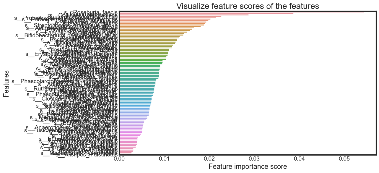
Feature Importance
Until now, I have used all the features given in the model. Now, I will select only the important features, build the model using these features and see its effect on accuracy.
feature_scores = pd.Series(rfc_final.feature_importances_,
                           index=x_train.columns,
                           name='Importance').sort_values(ascending=False)

feature_scores
s__Roseburia_faecis                    0.054408
s__Parvimonas_micra                    0.038683
s__Collinsella_aerofaciens             0.028716
s__Bacteroides_cellulosilyticus        0.022687
s__Proteobacteria_bacterium_CAG_139    0.021398
                                         ...
s__Clostridium_symbiosum               0.003134
s__Bacteroides_uniformis               0.003102
s__Bacteroides_coprocola               0.002990
s__Megamonas_hypermegale               0.002715
s__Alistipes_indistinctus              0.002612
Name: Importance, Length: 100, dtype: float64
f, ax = plt.subplots(figsize=(10, 6))
ax = sns.barplot(x=feature_scores, y=feature_scores.index)
ax.set_title("Visualize feature scores of the features")
ax.set_yticklabels(feature_scores.index)
ax.set_xlabel("Feature importance score")
ax.set_ylabel("Features")
plt.show()
Selecting features by importance
feature_scores.to_frame()
| Importance | |
|---|---|
| s__Roseburia_faecis | 0.054408 |
| s__Parvimonas_micra | 0.038683 |
| s__Collinsella_aerofaciens | 0.028716 |
| s__Bacteroides_cellulosilyticus | 0.022687 |
| s__Proteobacteria_bacterium_CAG_139 | 0.021398 |
| ... | ... |
| s__Clostridium_symbiosum | 0.003134 |
| s__Bacteroides_uniformis | 0.003102 |
| s__Bacteroides_coprocola | 0.002990 |
| s__Megamonas_hypermegale | 0.002715 |
| s__Alistipes_indistinctus | 0.002612 |
100 rows × 1 columns
selected_features_imp = feature_scores.to_frame()
selected_features_imp = selected_features_imp[selected_features_imp['Importance'] > 0.01]
selected_features_imp
| Importance | |
|---|---|
| s__Roseburia_faecis | 0.054408 |
| s__Parvimonas_micra | 0.038683 |
| s__Collinsella_aerofaciens | 0.028716 |
| s__Bacteroides_cellulosilyticus | 0.022687 |
| s__Proteobacteria_bacterium_CAG_139 | 0.021398 |
| s__Parasutterella_excrementihominis | 0.020249 |
| s__Coprobacter_fastidiosus | 0.019776 |
| s__Eubacterium_eligens | 0.019302 |
| s__Bacteroides_plebeius | 0.019007 |
| s__Streptococcus_anginosus_group | 0.018813 |
| s__Lachnospira_pectinoschiza | 0.018070 |
| s__Actinomyces_sp_HMSC035G02 | 0.016633 |
| s__Parabacteroides_goldsteinii | 0.016162 |
| s__Alistipes_shahii | 0.015669 |
| s__Faecalibacterium_prausnitzii | 0.015090 |
| s__Bacteroides_dorei | 0.014330 |
| s__Bifidobacterium_pseudocatenulatum | 0.014211 |
| s__Turicimonas_muris | 0.013414 |
| s__Roseburia_intestinalis | 0.013204 |
| s__Bacteroides_xylanisolvens | 0.012800 |
| s__Rothia_mucilaginosa | 0.012791 |
| s__Bifidobacterium_longum | 0.012468 |
| s__Streptococcus_mitis | 0.012383 |
| s__Mogibacterium_diversum | 0.011902 |
| s__Blautia_wexlerae | 0.011741 |
| s__Eubacterium_sulci | 0.011740 |
| s__Clostridium_clostridioforme | 0.011074 |
| s__Eubacterium_sp_CAG_38 | 0.011013 |
| s__Eubacterium_rectale | 0.010855 |
| s__Erysipelatoclostridium_ramosum | 0.010849 |
| s__Anaerostipes_hadrus | 0.010746 |
| s__Ruminococcus_lactaris | 0.010473 |
| s__Actinomyces_odontolyticus | 0.010403 |
| s__Clostridium_sp_CAG_58 | 0.010365 |
Rebuilding model
Using the selected features to rebuild the model
# dataset
X_rebuild = data_selected[selected_features_imp.index.to_list()]
Y = data['disease']

# data splition
x_train, x_test, y_train, y_test = train_test_split(
    X_rebuild, Y, test_size = 0.30, random_state = 42)
## Cleaning test sets to avoid future warning messages
y_train = y_train.values.ravel()
y_test = y_test.values.ravel()

# build model
rfc_rebuild = RandomForestClassifier(bootstrap = True,
                                     criterion = 'gini',
                                     max_features = 'auto',
                                     max_depth = 4,
                                     n_estimators = 200,
                                     random_state = 123)
rfc_rebuild.fit(x_train, y_train)

classifier_score_rebuild = rfc_rebuild.score(x_train, y_train)
print('\nThe classifier accuracy score is {:03.2f}\n'.format(classifier_score_rebuild))
The classifier accuracy score is 0.91
%%capture --no-display

%matplotlib inline
import matplotlib.pyplot as plt
from IPython.display import Image, display
from sklearn import metrics, preprocessing

predicted = rfc_rebuild.predict(x_test)
accuracy = accuracy_score(y_test, predicted)

cm = metrics.confusion_matrix(y_test, predicted)

fig, ax = plt.subplots(figsize=(5, 5))
ax.matshow(cm, cmap=plt.cm.Reds, alpha=0.3)
for i in range(cm.shape[0]):
     for j in range(cm.shape[1]):
         ax.text(x=j, y=i,
                s=cm[i, j],
                va='center', ha='center')
plt.xlabel('Predicted Values', )
plt.ylabel('Actual Values')

ax.set_xticklabels([''] + ['Healthy', "CRC"])
ax.set_yticklabels([''] + ['Healthy', "CRC"])

plt.show()
predictions_prob = rfc_rebuild.predict_proba(x_test)[:, 1]

fpr2, tpr2, _ = roc_curve(y_test,
                          predictions_prob,
                          pos_label = 1)

auc_rf = auc(fpr2, tpr2)

print("The AUC for model is: {0: .4f}" .format(auc_rf))

plot_roc_curve(fpr2, tpr2, auc_rf, 'rf',
               xlim=(-0.01, 1.05),
               ylim=(0.001, 1.05))
The AUC for model is: 0.6792
Summary
Random Forest classification predictive modeling from end-to-end using Python.
- Exploratory Data analysis.
- Feature selection.
- Tune Parameters.
- Performance Evaluation.
- The optimal features for rebuilding model.
- Finalize results