Optimizing the SVM Classifier
Notebook 7: Optimizing the Support Vector Classifier.
Machine learning models are parameterized so that their behavior can be tuned for a given problem. Models can have many parameters and finding the best combination of parameters can be treated as a search problem. In this notebook, I aim to tune parameters of the SVM Classification model using scikit-learn.
Loading libraries
%matplotlib inline
import matplotlib.pyplot as plt

#Load libraries for data processing
import pandas as pd
import numpy as np
from scipy.stats import norm

## Supervised learning.
from sklearn.preprocessing import StandardScaler
from sklearn.preprocessing import LabelEncoder
from sklearn.model_selection import train_test_split
from sklearn.svm import SVC
from sklearn.model_selection import cross_val_score
from sklearn.model_selection import GridSearchCV
from sklearn.pipeline import make_pipeline
from sklearn.metrics import confusion_matrix
from sklearn import metrics, preprocessing
from sklearn.metrics import classification_report
from sklearn.feature_selection import SelectKBest, f_regression

# visualization
import seaborn as sns
plt.style.use('fivethirtyeight')
sns.set_style("white")

plt.rcParams['figure.figsize'] = (8,4)
#plt.rcParams['axes.titlesize'] = 'large'
Importing data
'''
# raw data
data_df = pd.read_table('./dataset/MergeData.tsv', sep="\t", index_col=0)
data = data_df.reset_index(drop=True)
data.head()
# CLR-transformed data
data_df = pd.read_table('./dataset/MergeData_clr.tsv', sep="\t", index_col=0)
data = data_df.reset_index(drop=True)
data.head()
'''
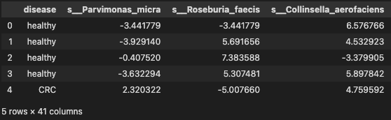
# significant species
data_df = pd.read_table('./dataset/MergeData_clr_signif.tsv', sep="\t", index_col=0)
data = data_df.reset_index(drop=True)
data.head()
Building a predictive model and evaluate with 5-cross validation using support vector classifies (ref Predictive model using Support Vector Machine) for details
#Assign predictors to a variable of ndarray (matrix) type
array = data.values
X = array[:, 1:data.shape[1]]
y = array[:, 0]
#transform the class labels from their original string representation (M and B) into integers
le = LabelEncoder()
y = le.fit_transform(y)
# Normalize the data (center around 0 and scale to remove the variance).
scaler = StandardScaler()
Xs = scaler.fit_transform(X)
from sklearn.decomposition import PCA
# feature extraction
pca = PCA(n_components=10)
fit = pca.fit(Xs)
X_pca = pca.transform(Xs)
# 5. Divide records in training and testing sets.
X_train, X_test, y_train, y_test = train_test_split(X_pca, y, test_size=0.3, random_state=2, stratify=y)
# 6. Create an SVM classifier and train it on 70% of the data set.
clf = SVC(probability=True)
clf.fit(X_train, y_train)
#7. Analyze accuracy of predictions on 30% of the holdout test sample.
classifier_score = clf.score(X_test, y_test)
print ('\nThe classifier accuracy score is {:03.2f}\n'.format(classifier_score))
clf2 = make_pipeline(SelectKBest(f_regression, k=3),SVC(probability=True))
scores = cross_val_score(clf2, X_pca, y, cv=3)
# Get average of 5-fold cross-validation score using an SVC estimator.
n_folds = 5
cv_error = np.average(cross_val_score(SVC(), X_pca, y, cv=n_folds))
#print ('\nThe {}-fold cross-validation accuracy score for this classifier is {:.2f}\n'.format(n_folds, cv_error))
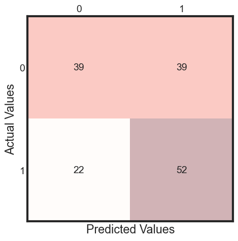
y_pred = clf.fit(X_train, y_train).predict(X_test)
cm = metrics.confusion_matrix(y_test, y_pred)
print(classification_report(y_test, y_pred ))
fig, ax = plt.subplots(figsize=(5, 5))
ax.matshow(cm, cmap=plt.cm.Reds, alpha=0.3)
for i in range(cm.shape[0]):
for j in range(cm.shape[1]):
ax.text(x=j, y=i,
s=cm[i, j],
va='center', ha='center')
plt.xlabel('Predicted Values', )
plt.ylabel('Actual Values')
plt.show()
The classifier accuracy score is 0.60

              precision    recall  f1-score   support

           0       0.64      0.50      0.56        78
           1       0.57      0.70      0.63        74

    accuracy                           0.60       152
   macro avg       0.61      0.60      0.60       152
weighted avg       0.61      0.60      0.59       152
Importance of optimizing a classifier
We can tune two key parameters of the SVM algorithm:
- the value of C (how much to relax the margin)
- and the type of kernel.
The default for SVM (the SVC class) is to use the Radial Basis Function (RBF) kernel with a C value set to 1.0. Like with KNN, we will perform a grid search using 10-fold cross validation with a standardized copy of the training dataset. We will try a number of simpler kernel types and C values with less bias and more bias (less than and more than 1.0 respectively).
Python scikit-learn provides two simple methods for algorithm parameter tuning:
- Grid Search Parameter Tuning.
- Random Search Parameter Tuning.
# Train classifiers.
kernel_values = [ 'linear' ,  'poly' ,  'rbf' ,  'sigmoid' ]
param_grid = {'C': np.logspace(-3, 2, 6), 'gamma': np.logspace(-3, 2, 6),'kernel': kernel_values}

grid = GridSearchCV(SVC(), param_grid=param_grid, cv=5)
grid.fit(X_train, y_train)
GridSearchCV(cv=5, estimator=SVC(),
             param_grid={'C': array([1.e-03, 1.e-02, 1.e-01, 1.e+00, 1.e+01, 1.e+02]),
                         'gamma': array([1.e-03, 1.e-02, 1.e-01, 1.e+00, 1.e+01, 1.e+02]),
                         'kernel': ['linear', 'poly', 'rbf', 'sigmoid']})
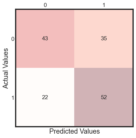
print("The best parameters are %s with a score of %0.2f"
      % (grid.best_params_, grid.best_score_))
The best parameters are {'C': 1.0, 'gamma': 0.001, 'kernel': 'rbf'} with a score of 0.69
grid.best_estimator_.probability = True
clf = grid.best_estimator_
y_pred = clf.fit(X_train, y_train).predict(X_test)
cm = metrics.confusion_matrix(y_test, y_pred)
#print(cm)
print(classification_report(y_test, y_pred ))

fig, ax = plt.subplots(figsize=(5, 5))
ax.matshow(cm, cmap=plt.cm.Reds, alpha=0.3)
for i in range(cm.shape[0]):
     for j in range(cm.shape[1]):
         ax.text(x=j, y=i,
                s=cm[i, j],
                va='center', ha='center')
plt.xlabel('Predicted Values', )
plt.ylabel('Actual Values')
plt.show()
              precision    recall  f1-score   support

           0       0.66      0.55      0.60        78
           1       0.60      0.70      0.65        74

    accuracy                           0.62       152
   macro avg       0.63      0.63      0.62       152
weighted avg       0.63      0.62      0.62       152
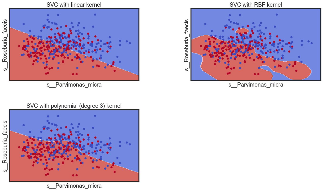
Decision boundaries of different classifiers
Let’s see the decision boundaries produced by the linear, Gaussian and polynomial classifiers.
- s__Parvimonas_micra
- s__Roseburia_faecis
import matplotlib.pyplot as plt
from matplotlib.colors import ListedColormap
from sklearn import svm, datasets

def decision_plot(X_train, y_train, n_neighbors, weights):
       h = .02  # step size in the mesh

Xtrain = X_train[:, :2] # we only take the first two features (s__Parvimonas_micra, s__Roseburia_faecis).

#================================================================
# Create color maps
#================================================================
cmap_light = ListedColormap(['#FFAAAA', '#AAFFAA', '#AAAAFF'])
cmap_bold = ListedColormap(['#FF0000', '#00FF00', '#0000FF'])


#================================================================
# we create an instance of SVM and fit out data.
# We do not scale ourdata since we want to plot the support vectors
#================================================================

C = 1.0  # SVM regularization parameter

svm = SVC(kernel='linear', random_state=0, gamma=0.1, C=C).fit(Xtrain, y_train)
rbf_svc = SVC(kernel='rbf', gamma=0.7, C=C).fit(Xtrain, y_train)
poly_svc = SVC(kernel='poly', degree=3, C=C).fit(Xtrain, y_train)
%matplotlib inline
plt.rcParams['figure.figsize'] = (15, 9)
plt.rcParams['axes.titlesize'] = 'large'

# create a mesh to plot in
x_min, x_max = Xtrain[:, 0].min() - 1, Xtrain[:, 0].max() + 1
y_min, y_max = Xtrain[:, 1].min() - 1, Xtrain[:, 1].max() + 1
xx, yy = np.meshgrid(np.arange(x_min, x_max, 0.1),
                         np.arange(y_min, y_max, 0.1))

# title for the plots
titles = ['SVC with linear kernel',
          'SVC with RBF kernel',
          'SVC with polynomial (degree 3) kernel']
for i, clf in enumerate((svm, rbf_svc, poly_svc)):
    # Plot the decision boundary. For that, we will assign a color to each
    # point in the mesh [x_min, x_max]x[y_min, y_max].
    plt.subplot(2, 2, i + 1)
    plt.subplots_adjust(wspace=0.4, hspace=0.4)

    Z = clf.predict(np.c_[xx.ravel(), yy.ravel()])

    # Put the result into a color plot
    Z = Z.reshape(xx.shape)
    plt.contourf(xx, yy, Z, cmap=plt.cm.coolwarm, alpha=0.8)

    # Plot also the training points
    plt.scatter(Xtrain[:, 0], Xtrain[:, 1], c=y_train, cmap=plt.cm.coolwarm)
    plt.xlabel('s__Parvimonas_micra')
    plt.ylabel('s__Roseburia_faecis')
    plt.xlim(xx.min(), xx.max())
    plt.ylim(yy.min(), yy.max())
    plt.xticks(())
    plt.yticks(())
    plt.title(titles[i])

plt.show()
Conclusion
This work demonstrates the modelling of CRC as classification task using Support Vector Machine
The SVM performs better when the dataset is standardized so that all attributes have a mean value of zero and a standard deviation of one. We can calculate this from the entire training dataset and apply the same transform to the input attributes from the validation dataset.
Next Task:
- Summary and conclusion of findings
- Compare with other classification methods
- Decision trees with tree.DecisionTreeClassifier();
- K-nearest neighbors with neighbors.KNeighborsClassifier();
- Random forests with ensemble.RandomForestClassifier();
- Perceptron (both gradient and stochastic gradient) with mlxtend.classifier.Perceptron; and
- Multilayer perceptron network (both gradient and stochastic gradient) with mlxtend.classifier.MultiLayerPerceptron.