Data clean
Notebook 2: Identifying the problem and Getting data.
Removing the unmathed samples or participants.
Identify the problem
Colorectal cancer (CRC), also known as bowel cancer, colon cancer, or rectal cancer, is the development of cancer from the colon or rectum (parts of the large intestine). Signs and symptoms may include blood in the stool, a change in bowel movements, weight loss, and fatigue. Gut microbiota play crucial role in CRC progression. Here, to investigate whether the gut microbiota could predict healthy control or CRC patients.
Expected outcome
Since this build a model that can classify healthy control or CRC patients using two training classification:
- CRC = Patients - Present
- healthy = Control - Absent
Objective
Since the labels in the data are discrete, the predication falls into two categories, (i.e. CRC or healthy). In machine learning this is a classification problem.
Thus, the goal is to classify healthy control or CRC patients. To achieve this we have used machine learning classification methods to fit a function that can predict the discrete class of new input.
Identify data sources
The datasets contains two files:
- metadata: The 1st and 2nd columns in the dataset store the unique ID numbers of the samples and disease (CRC=Patients, healthy=Control), respectively.
- profile: The gut microbial species level profile.
Loading libraries
import numpy as np
import pandas as pd
Importing Dataset
First, load the TSV and CSV file using read_table or read_csv function of Pandas, respectively
metadata = pd.read_csv("./dataset/metadata.csv", index_col=0)
profile = pd.read_table("./dataset/species.tsv", sep="\t")
Inspecting the data
The first step is to visually inspect datasets.
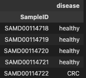
metadata.head()

profile.head()

Choosing only healthy or CRC samples
Selecting healthy or CRC samples to further data analysis
- filtering disease on metadata dataset
phen = metadata.loc[(metadata['disease'] == 'healthy') | (metadata['disease'] == 'CRC')]

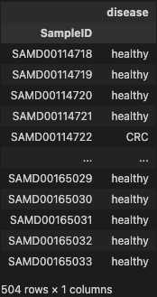
phen

- filtering the species with low occurrrence
profile_trim = profile[phen.index]
profile_trim.index = profile.TaxaID

prof = profile_trim[profile_trim.apply(lambda x: np.count_nonzero(x)/len(x), axis=1) > 0.2]
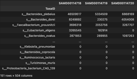
prof

The “info()” method provides a concise summary of the data; from the output, it provides the type of data in each column, the number of non-null values in each column, and how much memory the data frame is using.
The method get_dtype_counts() will return the number of columns of each type in a DataFrame:
# Review data types with "info()".
phen.info()
<class 'pandas.core.frame.DataFrame'>
Index: 504 entries, SAMD00114718 to SAMD00165033
Data columns (total 1 columns):
 #   Column   Non-Null Count  Dtype
---  ------   --------------  -----
 0   disease  504 non-null    object
dtypes: object(1)
memory usage: 7.9+ KB
# Review number of columns of each data type in a DataFrame:
phen.dtypes.value_counts()
object    1
dtype: int64
#check for missing variables
phen.isnull().any()
disease    False
dtype: bool
phen.disease.unique()
array(['healthy', 'CRC'], dtype=object)
From the results above, disease is a categorical variable, because it represents a fix number of possible values (i.e, disease. The machine learning algorithms wants numbers, and not strings, as their inputs so we need some method of coding to convert them.
Integrating the phen and prof data
Here, we select disease from phen and then integrate it with prof into new dataset for the downstream analysis
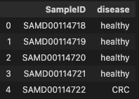
phen_cln = phen.iloc[:, 0].rename_axis("SampleID").reset_index()
phen_cln.head()

prof_cln = prof.T.rename_axis("SampleID").reset_index()
prof_cln.head()

mdat = pd.merge(phen_cln, prof_cln, on="SampleID", how="inner")
mdat.head()

#save the cleaner version of dataframe for future analyis
mdat.to_csv('./dataset/MergeData.tsv',
            sep='\t', encoding='utf-8', index=False)
Summary
- 151 species were selected more then 0.2 occurrence in Gastric Cancer
- 504 patients with Gastric Cancer were chosen