Obtaining inpudata
Rmarkdown 1: Downloading data.
Downloading datasets using curatedMetagenomicData, which contains the HUMANN or Metaphlan results.
Loading packages
knitr::opts_chunk$set(warning = FALSE)
library(dplyr)
library(tibble)
library(curatedMetagenomicData)
#library(curatedMetagenomicAnalyses)

# rm(list = ls())
options(stringsAsFactors = F)
options(future.globals.maxSize = 1000 * 1024^2)
Investigating potential response variables
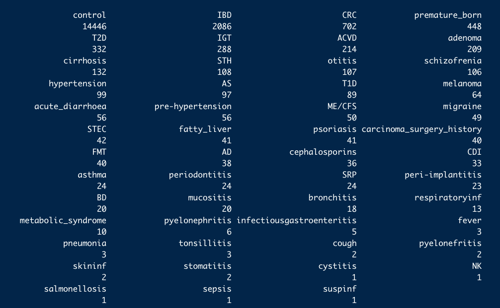
- These are the 10 study conditions most commonly found in curatedMetagenomicData:
data("sampleMetadata")
availablediseases <- pull(sampleMetadata, study_condition) %>%
  table() %>%
  sort(decreasing = TRUE)

availablediseases
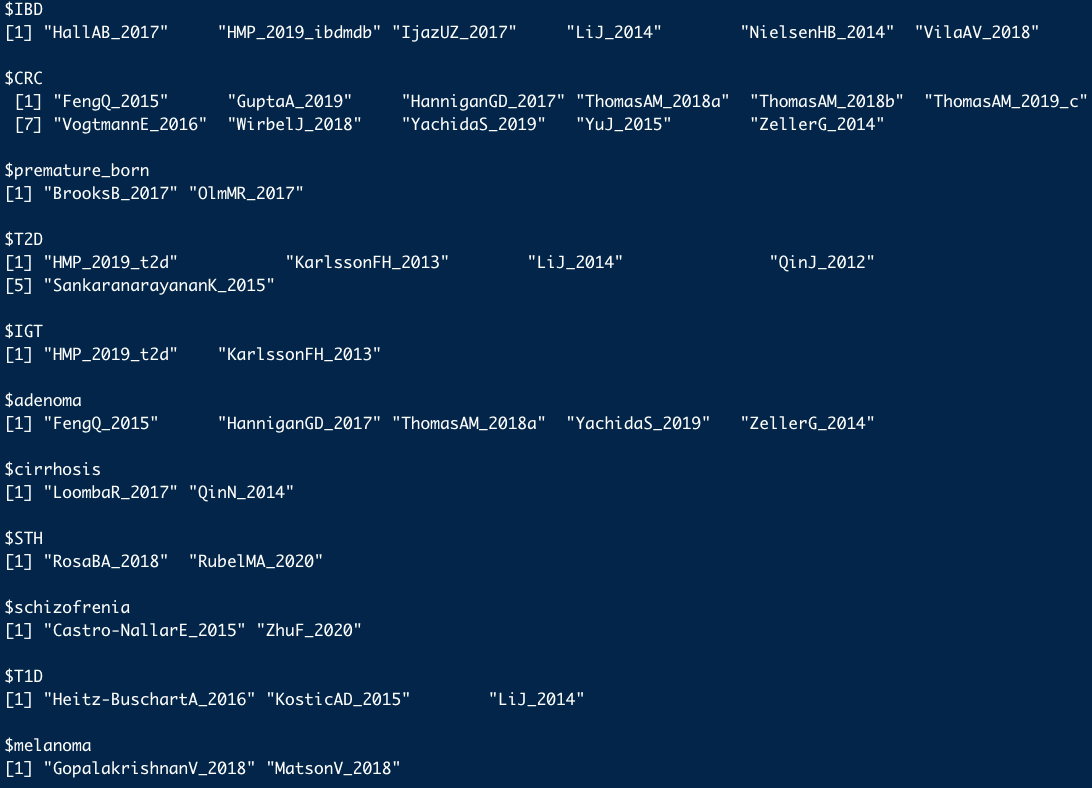
- And the number of studies they are found in:
studies <- lapply(names(availablediseases), function(x){
  filter(sampleMetadata, study_condition %in% x) %>%
    pull(study_name) %>%
    unique()
})
names(studies) <- names(availablediseases)
studies <- studies[-grep("control", names(studies))] #get rid of controls
studies <- studies[sapply(studies, length) > 1] #available in more than one study

studies
- Each of these datasets has six data types associated with it; for example:
curatedMetagenomicData(pattern = "YachidaS_2019.+",
                       dryrun = TRUE,
                       counts = TRUE,
                       rownames = "long")
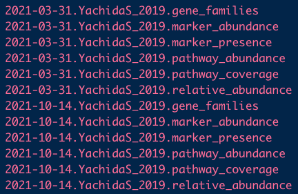
The metagenomics datasets contain more than 13 types data, which comprising taxonomic and functional profile with relative and absolute abundance matrix.
- Relative abundance: storing into TreeSummarizedExperiment object
YachidaS_2019_dataset <- curatedMetagenomicData(pattern = "YachidaS_2019.+relative_abundance",
                       dryrun = FALSE,
                       counts = TRUE,
                       rownames = "long")

YachidaS_2019_RB_TSE <- YachidaS_2019_dataset$`2021-10-14.YachidaS_2019.relative_abundance`
YachidaS_2019_RB_TSE
Write relative abundance datasets to disk
if (0) {
for (i in seq_along(studies)){
  cond <- names(studies)[i]
  se <-
    curatedMetagenomicAnalyses::makeSEforCondition(cond, removestudies = "HMP_2019_ibdmdb", dataType = "relative_abundance")
  print(paste("Next study condition:", cond, " /// Body site: ", unique(colData(se)$body_site)))
  print(with(colData(se), table(study_name, study_condition)))
  cat("\n \n")
  save(se, file = paste0(cond, ".rda"))
  flattext <- select(as.data.frame(colData(se)), c("study_name", "study_condition", "subject_id"))
  rownames(flattext) <- colData(se)$sample_id
  flattext <- cbind(flattext, data.frame(t(assay(se))))
  write.csv(flattext, file = paste0(cond, ".csv"))
  system(paste0("gzip ", cond, ".csv"))
}
}
Preparing for machine learning
metadata
relative abundance profile
metadata <- colData(YachidaS_2019_RB_TSE) %>%
  data.frame()
phenotype <- metadata %>%
  dplyr::select(disease) %>%
  tibble::rownames_to_column("SampleID") %>%
  dplyr::filter(disease %in% c("CRC", "healthy"))

profile <- assay(YachidaS_2019_RB_TSE)

sid <- intersect(phenotype$SampleID, colnames(profile))

prof <- profile %>%
  data.frame() %>%
  tibble::rownames_to_column("TaxaID") %>%
  dplyr::group_by(TaxaID) %>%
  dplyr::mutate(TaxaID_new = unlist(strsplit(TaxaID, "\\|"))[7]) %>%
  dplyr::select(TaxaID, TaxaID_new, all_of(sid)) %>%
  dplyr::ungroup() %>%
  dplyr::select(-TaxaID) %>%
  dplyr::rename(TaxaID = TaxaID_new)

phen <- phenotype %>%
  dplyr::filter(SampleID %in% sid)
output
if (!dir.exists("./dataset")) {
  dir.create("./dataset", recursive = TRUE)
}

write.csv(phen, "./dataset/metadata.csv", row.names = F)
write.table(prof, "./dataset/species.tsv", sep = "\t", quote = F, row.names = F)
Session info
devtools::session_info()